Improbable sequences of responses in the data

It seems that the original data has been first sorted per condition, and then that a “ResponseID” was assigned to participants. The data does not appear to be sorted on any other column or combination of columns.

When plotting the ReponseID against the number of cleansing-related words that people find, long sequences of repeated responses appear:

• A long streak of “0” appears in the Personal-Spontaneous condition (20)
• A long streak of “1” appears in the Personal-Instrumental condition (14)

ordata <- read.csv("originalData_cleaned.csv")

x <- ordata$content
y <- ordata$approach

ordata$conditions <- case_when(
  x == "professional" & y == "instrumental" ~ "prof - inst",
  x == "professional" & y == "spontaneous" ~ "prof - spont",
  x == "personal" & y == "instrumental" ~ "pers - inst",
  x == "personal" & y == "spontaneous" ~ "pers - spont",
)

options(repr.plot.width = 10, repr.plot.height = 4)
ggplot(ordata, aes(ResponseID, CWsum)) +
  geom_point(aes(colour = conditions), size = 1.25) +
  geom_mark_ellipse(data = ordata %>% 
                      filter(ResponseID >= 12 & ResponseID <= 31), colour = "blue", expand = unit(1, "mm")) +
  geom_mark_ellipse(data = ordata %>% 
                      filter(ResponseID >= 90 & ResponseID <= 103), colour = "blue", expand = unit(1, "mm")) +
  scale_y_continuous(breaks = c(0, 1, 2, 3), minor_breaks = NULL) +
  scale_x_continuous(breaks = seq(1, 306, 50)) +
  theme_classic() +
  ylab("Nber of cleansing-related words found")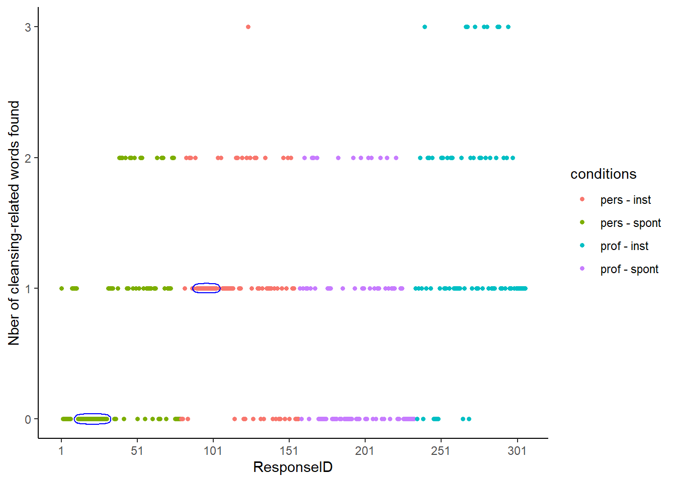

To determine the likelihood of these streaks emerging by chance alone, I repeatedly shuffled the data per condition, and constructed a distribution of possible “streak lengths”.

max_cons_value <- function(x, val) { # Function to compute longest streak of `val`
  y <- rle(x) # Rfunction rle for "run length encoding" (https://www.r-bloggers.com/2009/09/r-function-of-the-day-rle-2/)
  len <- y$lengths[y$value == val]
  max(len)
}

# Longest streaks observed in real data
sortedordata <- arrange(ordata, ResponseID)
maxgreen <- max_cons_value(sortedordata$CWsum, 0)
maxpink <- max_cons_value(sortedordata$CWsum, 1)

res_green <- ordata %>%
  # Vector of responses in the "green" condition
  arrange(ResponseID) %>%
  filter(conditions == "pers - spont") %>%
  pull(CWsum)

res_pink <- ordata %>%
  # Vector of responses in the "pink" condition
  arrange(ResponseID) %>%
  filter(conditions == "pers - inst") %>%
  pull(CWsum)

# Empty vectors to store shuffled results
outcome_g <- c()
outcome_p <- c()

nboots <- 10000

# Repeated shuffles
for (i in 1:nboots) {
  shuff <- sample(res_green) # Shuffle green responses
  maxseq <- max_cons_value(shuff, 0) # Longest sequence of zeros in shuffled vector
  outcome_g <- append(outcome_g, maxseq) # Store it

  shuff <- sample(res_pink) # Same for pink responses
  maxseq <- max_cons_value(shuff, 1)
  outcome_p <- append(outcome_p, maxseq)
}

green <- as.data.frame(outcome_g)
pink <- as.data.frame(outcome_p)

# 'p-values' of finding a streak at least this long
p_green <- sum(green$outcome_g >= maxgreen) / nboots
p_pink <- sum(pink$outcome_p >= maxpink) / nboots

# Plotting results

g1 <- ggplot(green, aes(outcome_g)) +
  geom_histogram(binwidth = 1, color = "darkgreen", fill = "palegreen") +
  geom_vline(aes(xintercept = maxgreen), color = "red", linetype = "dashed", size = 1) +
  scale_y_continuous(labels = function(x) paste0(x / nboots), breaks = seq(0, .35 * nboots, .05 * nboots), minor_breaks = NULL) +
  theme_bw() +
  xlab("Length of longest sequence of 0") +
  ylab("") +
  theme(aspect.ratio = 0.5) +
  ggtitle(str_glue("Personal - Spontaneous condition \n A sequence of 0 of length >= 20 \n is observed in {p_green} out of 10 000 shuffles")) +
  theme(plot.title = element_text(size = 10, hjust = 0.5))

g2 <- ggplot(pink, aes(outcome_p)) +
  geom_histogram(binwidth = 1, color = "deeppink4", fill = "lightpink1") +
  geom_vline(aes(xintercept = maxpink), color = "red", linetype = "dashed", size = 1) +
  scale_y_continuous(labels = function(x) paste0(x / nboots), breaks = seq(0, .3 * nboots, .05 * nboots), minor_breaks = NULL) +
  theme_bw() +
  xlab("Length of longest sequence of 1") +
  ylab("") +
  theme(aspect.ratio = 0.5) +
  ggtitle(str_glue("Personal - Instrumental condition \n A sequence of 1 of length >= 14 \n is observed less than {p_pink*100}% of 10 000 shuffles")) +
  theme(plot.title = element_text(size = 10, hjust = 0.5))

g1 + g2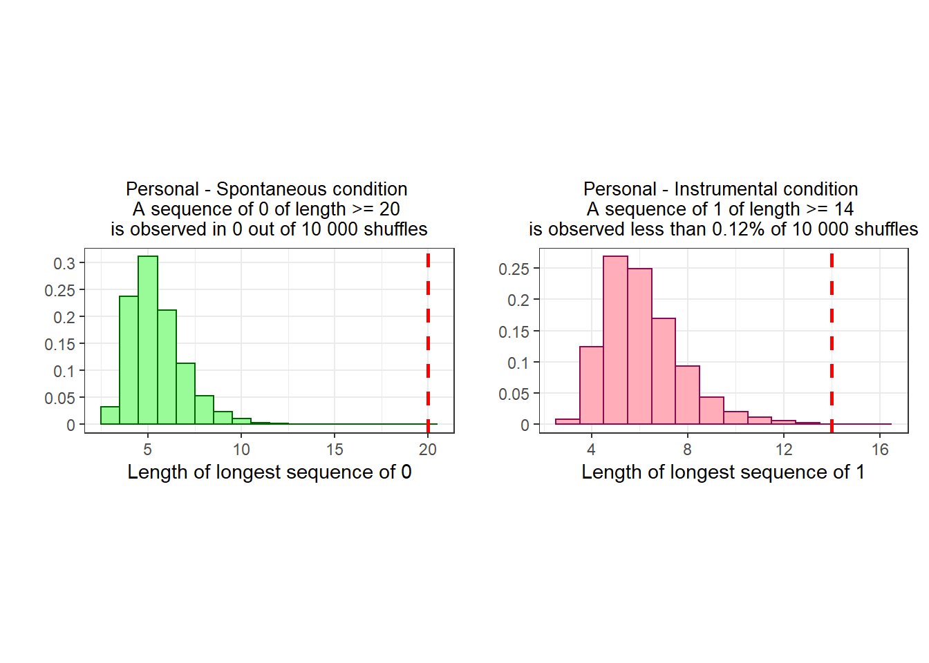

We find that these sequences are very unlikely to be caused by chance:

• A sequence of 20 or more zeroes never occurs.

• A sequence of 14 or more ones occurs 22 times out of 1 000 000.

Participants find different words in the replication (vs. original), but only on the ‘cleansing’ stems

When comparing the words generated for the non-cleansing stems (“F_O_”, “B_ _K”, and “PA_ _R”), there is no visible difference between the replication and the original study.

However, when looking at the words that people generate when they do not find the cleansing-related words, differences appear.

The figure below focuses on the trigrams of words that people find in the replication (vs. the original). For the cleansing stems, we focus on the participants who do not submit cleansing-related word (since otherwise the words that they submit are always the same).

The graph below shows all the trigrams that are present at least once in each dataset.

repdata <- read.csv("repData_cleaned.csv")

options(repr.plot.width = 12, repr.plot.height = 4)

rep <- repdata %>%
  select(CW1, CW2, CW3, CW1count, CW2count, CW3count, CWsum, condition) %>%
  mutate(type = "replication")

or <- ordata %>%
  select(CW1, CW2, CW3, CW1count, CW2count, CW3count, CWsum, approach) %>%
  rename(condition = approach) %>%
  mutate(type = "original")

cw <- rbind(rep, or)

cw_trigrams <- cw %>%
  filter(CWsum == 0) %>%
  mutate(combi2NCW = paste(CW1, CW2, CW3)) %>%
  add_count(type, combi2NCW, .drop = F) %>%
  complete(type, combi2NCW, fill = list(n = 0)) %>%
  group_by(combi2NCW) %>%
  filter(all(n >= 1))

trigrams <- ggplot(cw_trigrams, aes(x = fct_infreq(combi2NCW), fill = type)) +
  theme_classic() +
  ggtitle("Trigrams of words found on cleansing stems when participants find zero cleansing word") +
  xlab("") +
  ylab("") +
  geom_bar(mapping = aes(y = ..prop.., group = c(type)), position = position_dodge()) +
  theme(
    axis.text.x = element_text(angle = 90, vjust = 0.5, hjust = 1),
    plot.title = element_text(face = "bold", size = 10, hjust = 0.5, vjust = 0)
  ) +
  scale_fill_discrete(name = "Study")

trigrams

This chart shows large differences, for instance:

• “wish shake soup,” “with shiver soup,” “with shiner soup” are much more common in the replication.

• “with sheer soup” is seven times more common in the original. It is all the more surprising that “sheer” is an error (it does not match the stem “S H _ _ E R”).

As a placebo test, we can check if we observe similar discrepancies on the trigrams formed on the neutral stems. Since there are many more options, we restrict the graph to the trigrams that are found at least twice in each dataset.

options(repr.plot.width = 12, repr.plot.height = 4)

rep <- repdata %>%
  select(NW1, NW2, NW3) %>%
  mutate(type = "replication")

or <- ordata %>%
  select(NW1, NW2, NW3) %>%
  mutate(type = "original")

cw <- rbind(rep, or)

cw_trigrams_neutral <- cw %>%
  mutate(combiNeutral = paste(NW1, NW2, NW3)) %>%
  add_count(type, combiNeutral, .drop = F) %>%
  complete(type, combiNeutral, fill = list(n = 0)) %>%
  group_by(combiNeutral) %>%
  filter(all(n >= 2))

trigrams <- ggplot(cw_trigrams_neutral, aes(x = fct_infreq(combiNeutral), fill = type)) +
  theme_classic() +
  ggtitle("Trigrams of neutral words that people find on the neutral stems") +
  xlab("") +
  ylab("") +
  geom_bar(mapping = aes(y = ..prop.., group = c(type)), position = position_dodge()) +
  theme(
    axis.text.x = element_text(angle = 90, vjust = 0.5, hjust = 1),
    plot.title = element_text(face = "bold", size = 10, hjust = 0.5, vjust = 0)
  ) +
  scale_fill_discrete(name = "Study")

trigrams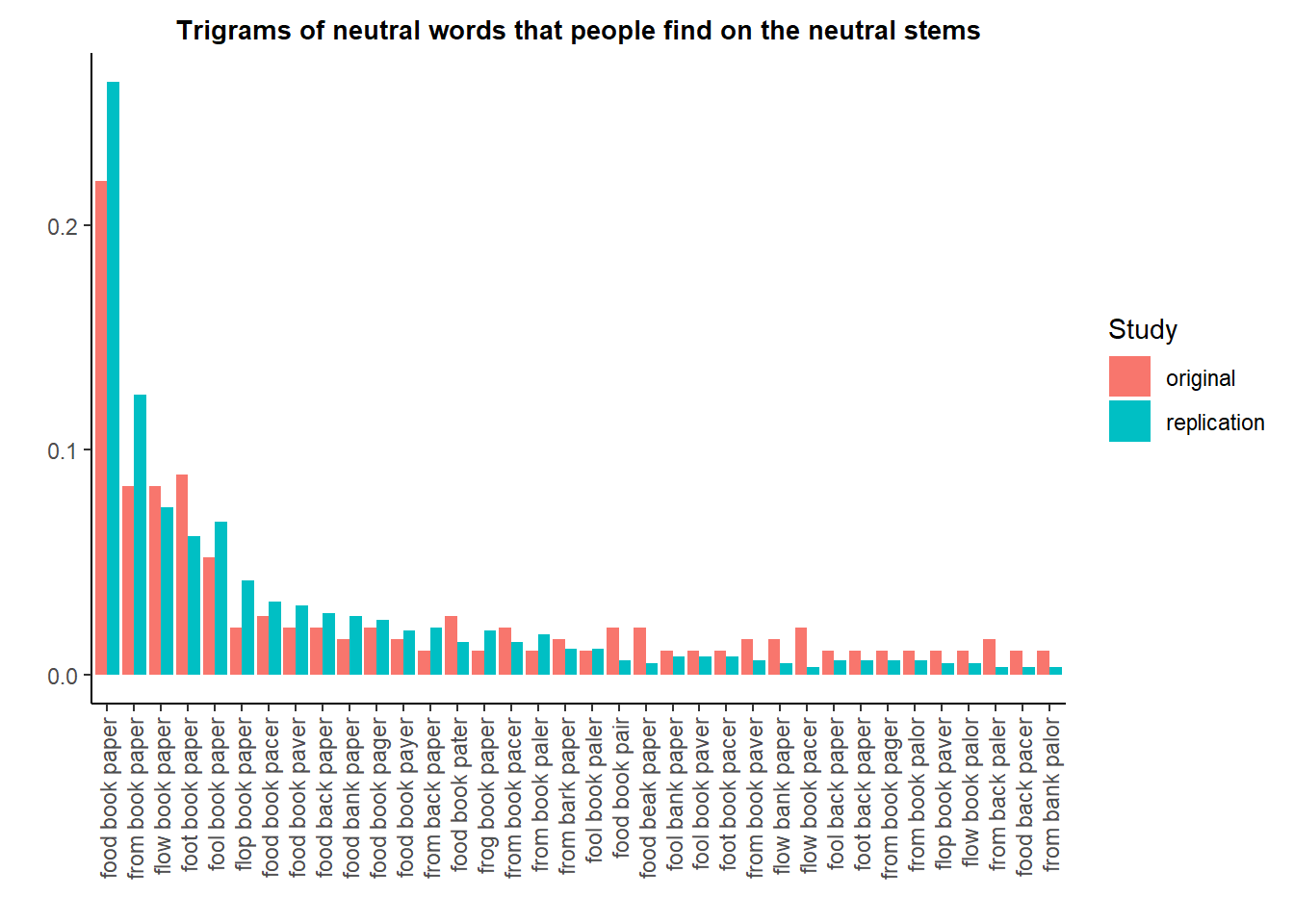

Here, the proportions appear very balanced.

To test if this dissimilarity is greater than what would be expected if the words came from a common population, we used the Cosine similarity of the words frequencies.

1. We consider the words written in the original and in the replication as two different “bags of words”.

2. We compare the frequencies of the words found in those two “bags of words” by computing their cosine similarity. The lower the cosine similarity, the more dissimilar the two “bags of words”.

3. We look how often we would find the two bags of words to be this dissimilar if we re-allocated the words at random between the original and the replication (i.e., if the two “bags of words” were drawn from the same distribution).

The graphs below present the results of this re-sampling procedure:

computecosinesim <- function(wordsbag1, wordsbag2) { # Function to compute cosine similarity
  listwords <- list(vec1 = wordsbag1, vec2 = wordsbag2)
  termcount <- table(stack(listwords))
  termf <- prop.table(termcount, 2)
  cosine(termf[, 1], termf[, 2])[1, 1]
}

rep <- repdata %>%
  select(CW1, NW1, CW2, NW2, CW3, NW3) %>%
  mutate(type = "replication")

or <- ordata %>%
  select(CW1, NW1, CW2, NW2, CW3, NW3) %>%
  mutate(type = "original")

# Dataframe of words
words <- rbind(rep, or) %>% mutate(
  CW1 = as.character(CW1), CW2 = as.character(CW2), CW3 = as.character(CW3),
  NW1 = as.character(NW1), NW2 = as.character(NW2), NW3 = as.character(NW3)
)

words_nowash <- words %>% filter(CW1 != "wash") # Words people find when they do not find 'wash'
words_noshower <- words %>% filter(CW2 != "shower") # Same for 'shower'
words_nosoap <- words %>% filter(CW3 != "soap") # Same for 'soap'

cwordsor <- c( # All words in original when people don't find the 'cleansing' words
  words_nowash %>%
    filter(type == "original") %>%
    pull(CW1),
  words_noshower %>% filter(type == "original") %>% pull(CW2),
  words_nosoap %>% filter(type == "original") %>% pull(CW3)
)

cwordsrep <- c( # All words in replication when people don't find the 'cleansing' words
  words_nowash %>%
    filter(type == "replication") %>%
    pull(CW1),
  words_noshower %>% filter(type == "replication") %>% pull(CW2),
  words_nosoap %>% filter(type == "replication") %>% pull(CW3)
)

# Observed similarity between the original and replication
obs_sim_clean <- computecosinesim(cwordsor, cwordsrep)

# Vector of labels
labels <- rep(c("original", "replication"), c(length(cwordsor), length(cwordsrep)))

# Vector of all words
wordsall <- c(cwordsor, cwordsrep)

coscoef <- c() # Empty vector of cosine similarities
for (i in 1:10000) {
  shufflabels <- sample(labels) # Shuffle the labels (i.e., original/replication)
  shuffor <- wordsall[shufflabels == "original"] # Select words in the new "original" data
  shuffrep <- wordsall[shufflabels == "replication"] # Select words in the new "replication" data
  bootsim <- computecosinesim(shuffor, shuffrep) # Cosine similarity of the shuffled words
  coscoef <- append(coscoef, bootsim) # Store it
}

# Create graph
cleansing <- as.data.frame(coscoef)
cleansingwords <- ggplot(cleansing, aes(coscoef)) +
  geom_histogram(binwidth = .0001, color = "palegreen4", fill = "palegreen1") +
  geom_vline(aes(xintercept = obs_sim_clean), color = "red", linetype = "dashed", size = 1) +
  scale_x_continuous(minor_breaks = NULL) +
  scale_y_continuous(minor_breaks = NULL) +
  theme_bw() +
  xlab("Cosine Similarity") +
  ylab("") +
  ggtitle("Cleansing Stems")

# We repeat same procedure for non-cleansing stems
nwordsor <- c(
  words %>% filter(type == "original") %>% pull(NW1),
  words %>% filter(type == "original") %>% pull(NW2),
  words %>% filter(type == "original") %>% pull(NW3)
)

nwordsrep <- c(
  words %>% filter(type == "replication") %>% pull(NW1),
  words %>% filter(type == "replication") %>% pull(NW2),
  words %>% filter(type == "replication") %>% pull(NW3)
)

# Observed similarity between the original and replication
obs_sim_neutral <- computecosinesim(nwordsor, nwordsrep)

# Vector of labels
labels <- rep(c("original", "replication"), c(length(nwordsor), length(nwordsrep)))

# Vector of all words
wordsall <- c(nwordsor, nwordsrep)

coscoef <- c() # Empty vector of cosine similarities
for (i in 1:10000) {
  shufflabels <- sample(labels) # Shuffle the labels (i.e., original/replication)
  shuffor <- wordsall[shufflabels == "original"] # Select words in the new "original" data
  shuffrep <- wordsall[shufflabels == "replication"] # Select words in the new "replication" data
  bootsim <- computecosinesim(shuffor, shuffrep) # Cosine similarity of the shuffled words
  coscoef <- append(coscoef, bootsim) # Store it
}

# Create graph
neutral <- as.data.frame(coscoef)
noncleansingwords <- ggplot(neutral, aes(coscoef)) +
  geom_histogram(binwidth = .0001, color = "navyblue", fill = "royalblue2") +
  geom_vline(aes(xintercept = obs_sim_neutral), color = "red", linetype = "dashed", size = 1) +
  scale_x_continuous(minor_breaks = NULL) +
  scale_y_continuous(minor_breaks = NULL) +
  theme_bw() +
  xlab("Cosine Similarity") +
  ylab("") +
  ggtitle("Non-cleansing Stems")

# Combine graphs
options(repr.plot.width = 10, repr.plot.height = 5)
cleansingwords + noncleansingwords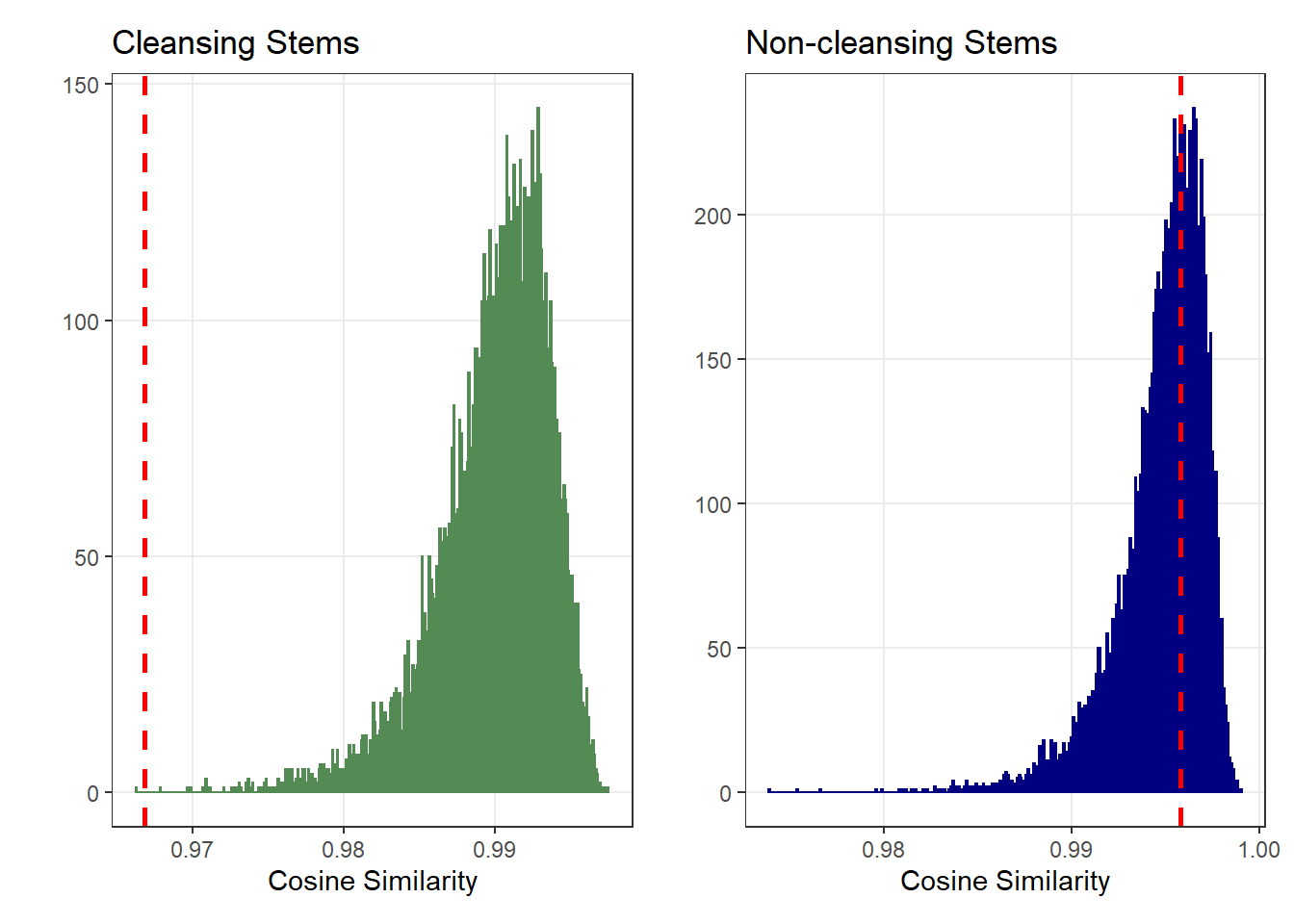

This confirms the visual observation:

When participants do not find cleansing-related words, they find different words in the Original (vs. Replication): The word frequencies are much more dissimilar than expected from random chance.

In contrast, the words that they find on the filler items are about as similar as expected between the Original and Replication.

This difference is not explained by the fact that the two studies use different conditions: We find the same result when restricting the analysis to the two conditions that are identical in both studies (professional - spontaneous vs. professional - instrumental).

Conclusion

These anomalies (improbable sequences of consecutive 0 or 1 in participants’ responses and participants who find different words in the replication compared with the original, but only on the cleansing stems), combined with the failure to replicate the effect, strongly suggest that the integrity of the data has been compromised.