Anomalies in Gino, Kouchaki, Casciaro 2020
library(tidyverse)
library(effsize)
library(ggbeeswarm)
library(vader)
The data of three studies are posted on the OSF. Study 1 is a correlational study, and study 3A and 3B are two experimental studies. We only focus on study 3A and 3B.
Description of Studies
- Study 3A
- Sample: MTurk, 599 participants
- 3 conditions: control vs. promotion focus vs. prevention focus
- Manipulation: writing task manipulating regulatory focus
- Task: participants read a story describing someone networking and are asked to put themselves in the shoes of the person described.
- Mediator: dirtiness on 7 items (dirty, inauthentic, impure, ashamed, wrong, unnatural, tainted), each measured on a 7-point scale
- DV: networking intentions on 4 items, each measured on a 7-point scale
- Study 3B
- Sample: MTurk, 572 participants
- Identical design, except for the task: participants had to “write an email” to a LinkedIn contact, instead of reading a story about networking.
Anomaly 1: similarity of effect sizes
The authors investigate the impact of regulatory focus on two variables:
Moral Impurity, a “proximal” variable in the hypothesized causal chain.
Networking Intensity, a “distal” variable in the hypothesized causal chain.
We might reasonably expect the effect on the “distal” variable (i.e., networking intentions) to be smaller than the impact on the “proximal” variable (i.e., moral impurity).
Instead, the effect sizes of the two comparisons reported in the paper (prevention vs. control and prevention vs. promotion) yield remarkably similar effects on both variables. In fact, the effect size on the “distal” variable (networking intensity) is directionally larger in both studies:
data3a <- read.csv("GKC2020_study3A_cleaned.csv")
data3b <- read.csv("GKC2020_study3B_cleaned.csv")

datacontrast <- data3a %>%
  filter(conditions %in% c("prevention", "promotion")) %>%
  mutate(conditions = as.factor(conditions),
         conditions = droplevels(conditions))
es1 <- cohen.d(MI ~ conditions, data = datacontrast)

datacontrast <- data3a %>%
  filter(conditions %in% c("prevention", "control")) %>%
  mutate(conditions = as.factor(conditions),
         conditions = droplevels(conditions))
es2 <- cohen.d(MI ~ conditions, data = datacontrast)

datacontrast <- data3a %>%
  filter(conditions %in% c("prevention", "promotion")) %>%
  mutate(conditions = as.factor(conditions),
         conditions = droplevels(conditions))
es3 <- cohen.d(NI ~ conditions, data = datacontrast)

datacontrast <- data3a %>%
  filter(conditions %in% c("prevention", "control")) %>%
  mutate(conditions = as.factor(conditions),
         conditions = droplevels(conditions))
es4 <- cohen.d(NI ~ conditions, data = datacontrast)

df <- data.frame(
  DV = rep(c("MI", "NI"), each = 2),
  Contrast = rep(c("promotion vs. prevention", "control vs. prevention"), times = 2),
  Effect_size = round(abs(c(es1$estimate, es2$estimate, es3$estimate, es4$estimate)), 3)
)

options(repr.plot.width = 6, repr.plot.height = 3)
ggplot(df, aes(Contrast, Effect_size)) +
  geom_point(aes(colour = factor(DV)), size = 2) +
  ylab("Effect size") +
  theme_classic() +
  theme(
    plot.title = element_text(hjust = 0.5, size = 12, face = "bold"),
    axis.title.x = element_text(size = 10, face = "bold"), axis.text.x = element_text(size = 8),
    axis.title.y = element_text(size = 10, face = "bold"), axis.text.y = element_text(size = 8),
    legend.title = element_text(size = 10, face = "bold"), legend.text = element_text(size = 8)
  ) +
  ggtitle("Study 3A") +
  scale_colour_discrete(name = "Dependent variable", labels = c("Moral impurity", "Networking intentions")) +
  scale_y_continuous(breaks = seq(0.3, 0.7, 0.05), minor_breaks = NULL)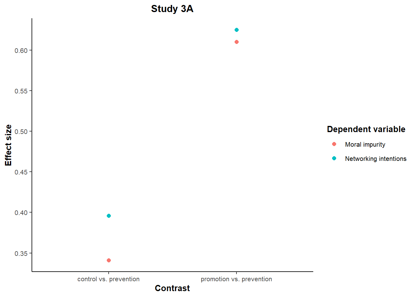
datacontrast <- data3b %>%
  filter(conditions %in% c("prevention", "promotion")) %>%
  mutate(conditions = as.factor(conditions),
         conditions = droplevels(conditions))
es1 <- cohen.d(MI ~ conditions, data = datacontrast)

datacontrast <- data3b %>%
  filter(conditions %in% c("prevention", "control")) %>%
  mutate(conditions = as.factor(conditions),
         conditions = droplevels(conditions))
es2 <- cohen.d(MI ~ conditions, data = datacontrast)

datacontrast <- data3b %>%
  filter(conditions %in% c("prevention", "promotion")) %>%
  mutate(conditions = as.factor(conditions),
         conditions = droplevels(conditions))
es3 <- cohen.d(NI ~ conditions, data = datacontrast)

datacontrast <- data3b %>%
  filter(conditions %in% c("prevention", "control")) %>%
  mutate(conditions = as.factor(conditions),
         conditions = droplevels(conditions))
es4 <- cohen.d(NI ~ conditions, data = datacontrast)

df <- data.frame(
  DV = rep(c("MI", "NI"), each = 2),
  Contrast = rep(c("promotion vs. prevention", "control vs. prevention"), times = 2),
  Effect_size = round(abs(c(es1$estimate, es2$estimate, es3$estimate, es4$estimate)), 3)
)

options(repr.plot.width = 6, repr.plot.height = 3)

ggplot(df, aes(Contrast, Effect_size)) +
  geom_point(aes(colour = factor(DV)), size = 2) +
  ylab("Effect size") +
  theme_classic() +
  theme(
      plot.title = element_text(hjust = 0.5, size = 12, face = "bold"),
    axis.title.x = element_text(size = 10, face = "bold"), axis.text.x = element_text(size = 8),
    axis.title.y = element_text(size = 10, face = "bold"), axis.text.y = element_text(size = 8),
    legend.title = element_text(size = 10, face = "bold"), legend.text = element_text(size = 8)
  ) + ggtitle("Study 3B") +
  scale_colour_discrete(name = "Dependent variable", labels = c("Moral impurity", "Networking intentions")) +
  scale_y_continuous(breaks = seq(0.2, 0.7, 0.05), minor_breaks = NULL)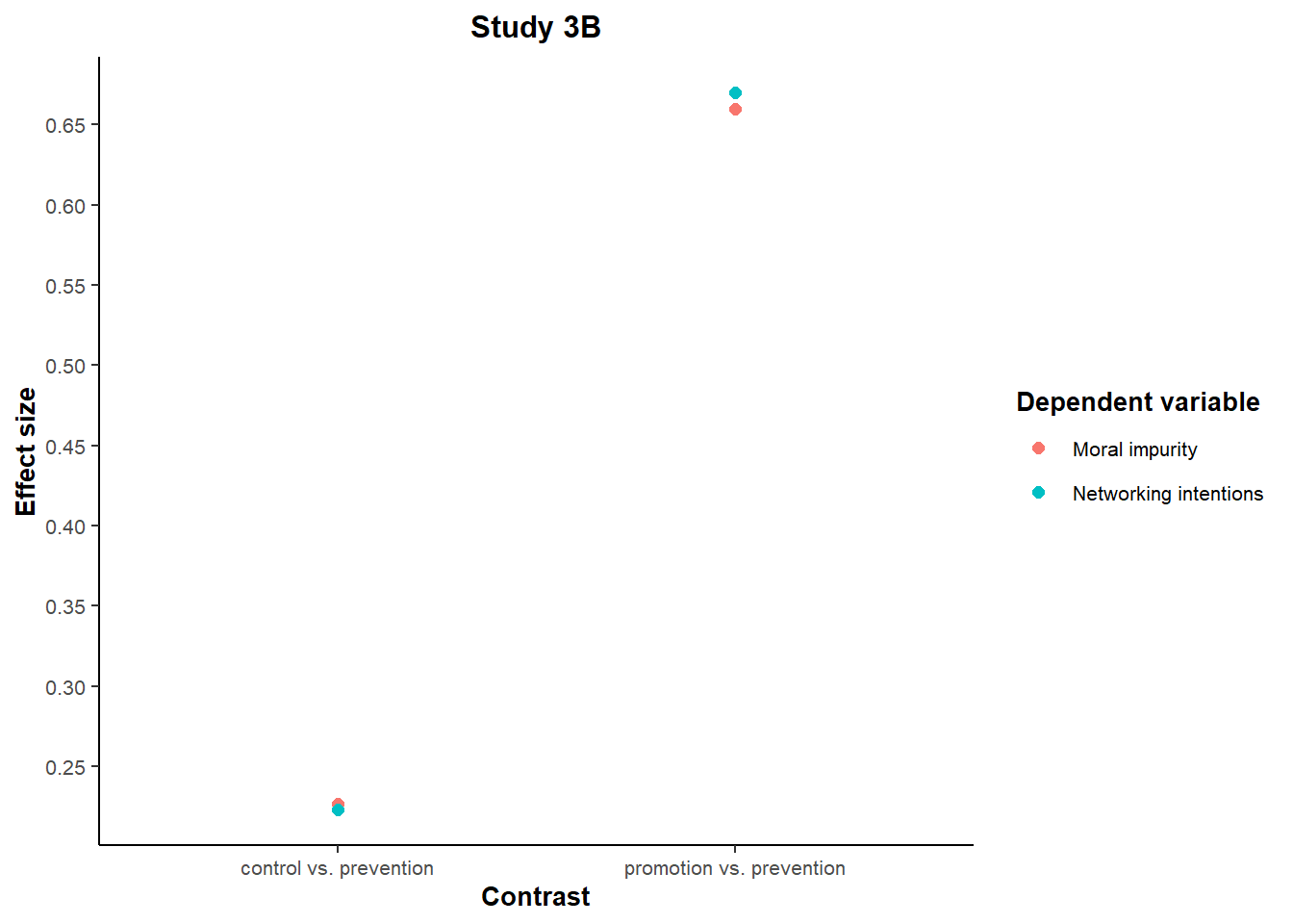
In addition, the effect sizes also appear more similar than expected for two variables sharing a weak correlation (-0.40 in study 3a and -0.32 in study 3b): Given the sampling variability inherent to any study, you might expect a larger difference between them.
To establish a benchmark on the degree of similarity that we should expect by random chance, we bootstrapped 10,000 samples from the data, and computed in each bootstrapped sample:
The absolute difference in the Cohen’s d of Prevention vs. Control on Moral Impurity (MI) and Networking Intentions (NI):
| d(MI, Prev vs. Control) - d(NI, Prev vs. Control) |The absolute difference in the Cohen’s d of Prevention vs. Promotion on Moral Impurity (MI) and Networking Intentions (NI):
| d(MI, Prev vs. Prom) - d(NI, Prev vs. Prom) |
The sum of these absolute differences forms the metric of (dis)similarity. We then compare the observed dissimilarity in the data to the distribution of dissimilarity in the 10,000 bootstrapped samples:
# Function that computes the sum of the absolute difference between effect sizes for each DV and each contrast
compute_dissimilarities <- function(NI_c, NI_prom, NI_prev, MI_c, MI_prom, MI_prev) {

  # effect sizes for each DV (NI and MI) and each contrast (prevention vs. control and prevention vs. promotion)
  es <- cohen.d(NI_c, NI_prev)
  dNI_PrevCt <- abs(es$estimate)

  es <- cohen.d(NI_prom, NI_prev)
  dNI_PrevProm <- abs(es$estimate)

  es <- cohen.d(MI_c, MI_prev)
  dMI_PrevCt <- abs(es$estimate)

  es <- cohen.d(MI_prom, MI_prev)
  dMI_PrevProm <- abs(es$estimate)

  # absolute difference between effect sizes: when diff = 0, perfect overlap between effect sizes
  diff_PrevCt <- abs(dNI_PrevCt - dMI_PrevCt)
  diff_PrevProm <- abs(dNI_PrevProm - dMI_PrevProm)

sum_of_diff <- diff_PrevCt + diff_PrevProm
  return(sum_of_diff)
}

# Applies the previous function on observed data
# values of NI and MI for each condition

ni_ctrl <- (data3a %>% filter(conditions == "control"))$NI
mi_ctrl <- (data3a %>% filter(conditions == "control"))$MI

ni_prom <- (data3a %>% filter(conditions == "promotion"))$NI
mi_prom <- (data3a %>% filter(conditions == "promotion"))$MI

ni_prev <- (data3a %>% filter(conditions == "prevention"))$NI
mi_prev <- (data3a %>% filter(conditions == "prevention"))$MI

# observed dissimilarity
obs_dissim3a <- compute_dissimilarities(ni_ctrl, ni_prom, ni_prev, mi_ctrl, mi_prom, mi_prev)

# Retrieves the sample size per condition
nber_ctrl <- length(ni_ctrl)
nber_prom <- length(ni_prom)
nber_prev <- length(ni_prev)

# Bootstrapping
# creation of an empty vector to which we will add the bootstrapped differences in effect sizes

boot_sim_es3a <- c()
for (i in 1:10000) {
  # selection of x indices (x = size of the sample per condition) with replacement in each condition
  bootind_ctrl <- sample.int(size = nber_ctrl, n = nber_ctrl, replace = TRUE)
  bootind_prom <- sample.int(size = nber_prom, n = nber_prom, replace = TRUE)
  bootind_prev <- sample.int(size = nber_prev, n = nber_prev, replace = TRUE)

  # retrieves the values associated with each index in each condition
  values1 <- ni_ctrl[bootind_ctrl]
  valuesA <- mi_ctrl[bootind_ctrl]

  values2 <- ni_prom[bootind_prom]
  valuesB <- mi_prom[bootind_prom]

  values3 <- ni_prev[bootind_prev]
  valuesC <- mi_prev[bootind_prev]

  # applies the previous function to compute for values selected in each condition on each DV the difference between effect sizes
  dissim <- compute_dissimilarities(values1, values2, values3, valuesA, valuesB, valuesC)

    # store the results
  boot_sim_es3a <- append(boot_sim_es3a, dissim)
}

bootp <- mean(boot_sim_es3a <= obs_dissim3a)

ggplot(as.data.frame(boot_sim_es3a), aes(x = boot_sim_es3a)) +
  geom_histogram(aes(y = ..count.. / sum(..count..), fill = "Bootstrapped"), bins = 100, color = "darkblue") +
  geom_vline(aes(color = "Observed", xintercept = obs_dissim3a), linetype = "dashed") +
  theme_bw() +
  ggtitle(str_glue("Study 3A \n This level of similarity is only observed \n in {bootp*100}% of the bootstrapped samples")) +
  xlab("Dissimilarity of Cohen's ds") +
  ylab("Probability") +
  theme(
    plot.title = element_text(hjust = 0.5, size = 10, face = "bold"),
    axis.title.x = element_text(size = 10, face = "bold"), axis.text.x = element_text(size = 8),
    axis.title.y = element_text(size = 10, face = "bold"), axis.text.y = element_text(size = 8)
  ) +
  scale_color_manual(name = "", values = c("Observed" = "Red")) +
  scale_fill_manual(name = "", values = c("Bootstrapped" = "lightblue")) +
  scale_y_continuous(minor_breaks = NULL)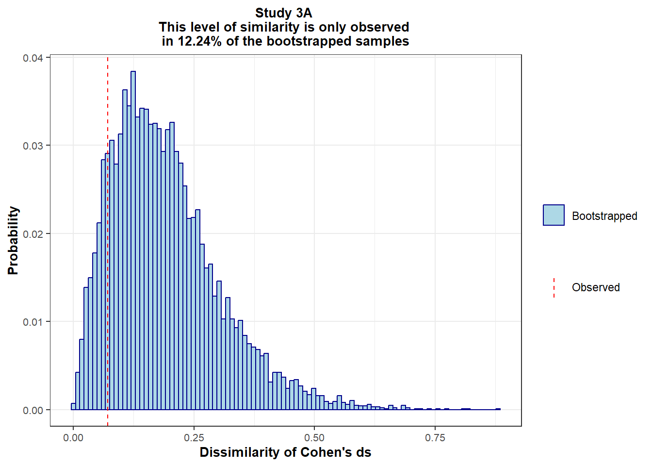
# Same procedure for Study 3B

ni_ctrl <- (data3b %>% filter(conditions == "control"))$NI
mi_ctrl <- (data3b %>% filter(conditions == "control"))$MI

ni_prom <- (data3b %>% filter(conditions == "promotion"))$NI
mi_prom <- (data3b %>% filter(conditions == "promotion"))$MI

ni_prev <- (data3b %>% filter(conditions == "prevention"))$NI
mi_prev <- (data3b %>% filter(conditions == "prevention"))$MI

# observed dissimilarity
obs_dissim3b <- compute_dissimilarities(ni_ctrl, ni_prom, ni_prev, mi_ctrl, mi_prom, mi_prev)

# Retrieves the sample size per condition
nber_ctrl <- length(ni_ctrl)
nber_prom <- length(ni_prom)
nber_prev <- length(ni_prev)

# Bootstrapping
# creation of an empty vector to which I will add the bootstrapped differences in effect sizes

boot_sim_es3b <- c()
for (i in 1:10000) {
  # selection of x indices (x = size of the sample per condition) with replacement in each condition
  bootind_ctrl <- sample.int(size = nber_ctrl, n = nber_ctrl, replace = TRUE)
  bootind_prom <- sample.int(size = nber_prom, n = nber_prom, replace = TRUE)
  bootind_prev <- sample.int(size = nber_prev, n = nber_prev, replace = TRUE)

  # retrieves the values associated with each index in each condition
  values1 <- ni_ctrl[bootind_ctrl]
  valuesA <- mi_ctrl[bootind_ctrl]

  values2 <- ni_prom[bootind_prom]
  valuesB <- mi_prom[bootind_prom]

  values3 <- ni_prev[bootind_prev]
  valuesC <- mi_prev[bootind_prev]

  # applies the previous function to compute for values selected in each condition on each DV the difference between effect sizes
  dissim <- compute_dissimilarities(values1, values2, values3, valuesA, valuesB, valuesC)

    # store the results
  boot_sim_es3b <- append(boot_sim_es3b, dissim)
}

bootp <- mean(boot_sim_es3b <= obs_dissim3b)

ggplot(as.data.frame(boot_sim_es3b), aes(x = boot_sim_es3b)) +
  geom_histogram(aes(y = ..count.. / sum(..count..), fill = "Bootstrapped"), bins = 100, color = "darkblue") +
  geom_vline(aes(color = "Observed", xintercept = obs_dissim3b), linetype = "dashed") +
  theme_bw() +
  ggtitle(str_glue("Study 3B \n This level of similarity is only observed \n in {bootp*100}% of the bootstrapped samples")) +
  xlab("Dissimilarity of Cohen's ds") +
  ylab("Probability") +
  theme(
    plot.title = element_text(hjust = 0.5, size = 10, face = "bold"),
    axis.title.x = element_text(size = 10, face = "bold"), axis.text.x = element_text(size = 8),
    axis.title.y = element_text(size = 10, face = "bold"), axis.text.y = element_text(size = 8)
  ) +
  scale_color_manual(name = "", values = c("Observed" = "Red")) +
  scale_fill_manual(name = "", values = c("Bootstrapped" = "lightblue")) +
  scale_y_continuous(minor_breaks = NULL)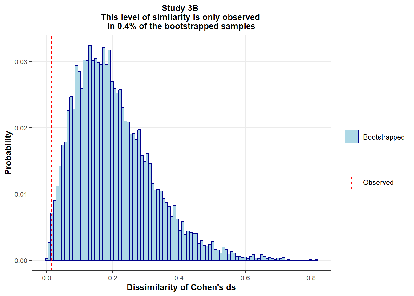
This simulation suggests that the similarity in effect sizes observed on the two variables is:
High in Study 3A, but compatible with what would be expected by chance.
Too high in Study 3B, and rarely compatible with what would be expected by chance.
Ultimately, the combined chance of randomly obtaining this high level of similarity in two independent studies is very small:
# Average bootstrapped similarity across data
avg_boot_sims <- (boot_sim_es3a + boot_sim_es3b) / 2

# Average observed similarity of effect sizes across data
avg_obs_sim <- (obs_dissim3a + obs_dissim3b) / 2

# Percentage of time this level of similalrity is observed in the bootstrapped samples
bootp <- mean(avg_boot_sims <= avg_obs_sim)

# Plotting the data
ggplot(as.data.frame(avg_boot_sims), aes(x = avg_boot_sims)) +
  geom_histogram(aes(y = ..count.. / sum(..count..), fill = "Bootstrapped"), bins = 100, color = "darkblue") +
  geom_vline(aes(color = "Observed", xintercept = avg_obs_sim), linetype = "dashed") +
  theme_bw() +
  ggtitle(str_glue("This level of similarity is only observed in two independent studies \n in {bootp*100}% of the bootstrapped samples")) +
  xlab("Dissimilarity of Cohen's ds") +
  ylab("Probability") +
  theme(
    plot.title = element_text(hjust = 0.5, size = 10, face = "bold"),
    axis.title.x = element_text(size = 10, face = "bold"), axis.text.x = element_text(size = 8),
    axis.title.y = element_text(size = 10, face = "bold"), axis.text.y = element_text(size = 8)
  ) +
  scale_color_manual(name = "", values = c("Observed" = "Red")) +
  scale_fill_manual(name = "", values = c("Bootstrapped" = "lightblue")) +
  scale_y_continuous(minor_breaks = NULL)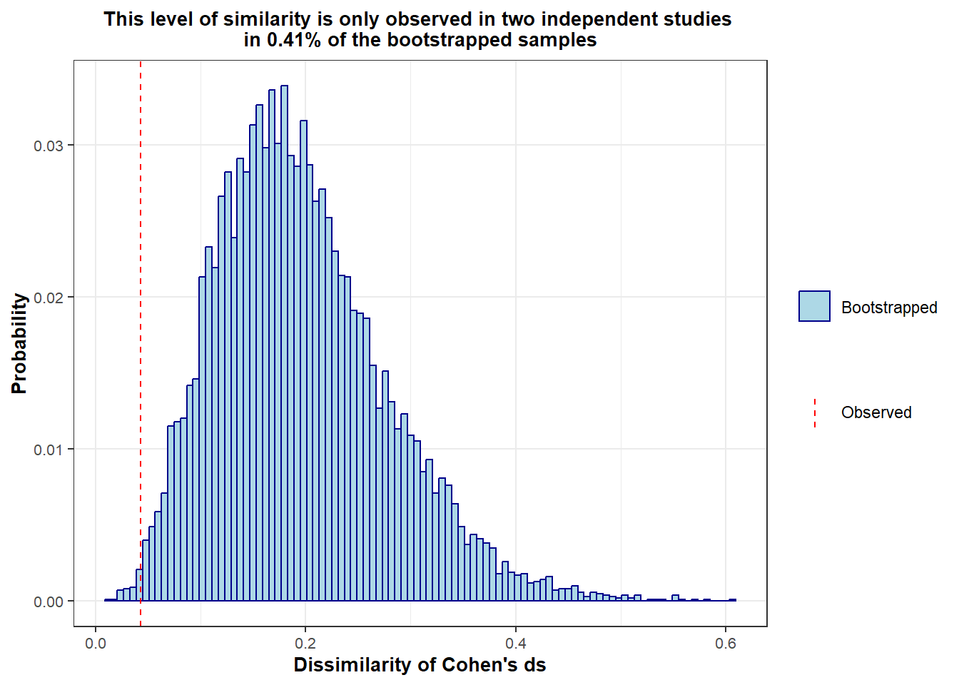
Anomaly 2: bunching on moral impurity
data3a <- data3a %>%
  rowwise() %>%
  mutate(sdMI = sd(c(MI1, MI2, MI3, MI4, MI5, MI6, MI7))) %>%
  as.data.frame()

data3a <- data3a %>% mutate(MIsingleanswer = ifelse(sdMI == 0, T, F))

ggplot(data = data3a, aes(x = conditions, y = MI, col = MIsingleanswer)) +
  geom_beeswarm(size = 1, cex = 0.3) +
  theme_bw() +
  ggtitle("Study 3A") +
  labs(
    x = "Conditions",
    y = "Moral impurity"
  ) +
  theme(
    plot.title = element_text(hjust = 0.5, size = 12, face = "bold"),
    axis.title.x = element_text(size = 10, face = "bold"), axis.text.x = element_text(size = 8),
    axis.title.y = element_text(size = 10, face = "bold"), axis.text.y = element_text(size = 8),
    legend.title = element_text(size = 8, face = "bold"), legend.text = element_text(size = 6)
  ) +
  scale_y_continuous(breaks = seq(1, 7, 1), minor_breaks = NULL) +
  scale_colour_discrete(name = "Same answer across items")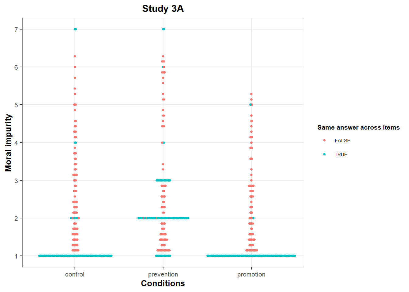
data3b <- data3b %>%
  rowwise() %>%
  mutate(sdMI = sd(c(MI1, MI2, MI3, MI4, MI5, MI6, MI7))) %>%
  as.data.frame()

data3b <- data3b %>% mutate(MIsingleanswer = ifelse(sdMI == 0, T, F))

ggplot(data = data3b, aes(x = conditions, y = MI, col = MIsingleanswer)) +
  geom_beeswarm(size = .8, cex = .15) +
  theme_bw() +
  ggtitle("Study 3B") +
  labs(
    x = "Conditions",
    y = "Moral impurity"
  ) +
  theme(
    plot.title = element_text(hjust = 0.5, size = 12, face = "bold"),
    axis.title.x = element_text(size = 10, face = "bold"), axis.text.x = element_text(size = 8),
    axis.title.y = element_text(size = 10, face = "bold"), axis.text.y = element_text(size = 8),
    legend.title = element_text(size = 8, face = "bold"), legend.text = element_text(size = 6),
  ) +
  scale_y_continuous(breaks = seq(1, 7, 1), minor_breaks = NULL) +
  scale_colour_discrete(name = "Same answer across items") +
  scale_x_discrete(expand = c(0.1, 0.1))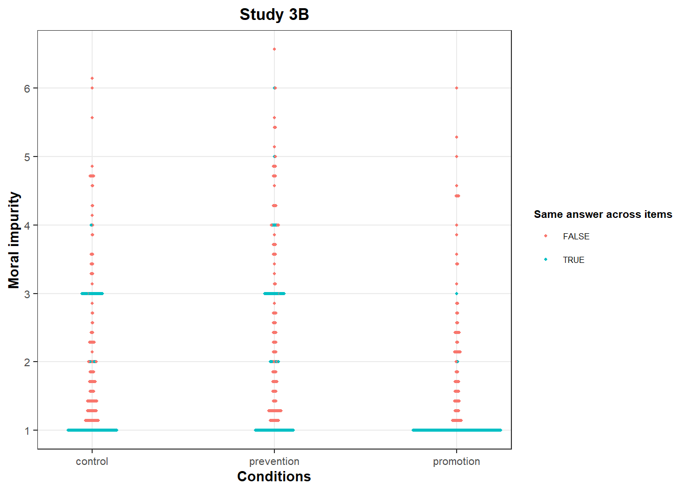
In all conditions, there are many “all 1s” responses on the “Moral Impurity” scale. This is typical of a floor effect: People would like to answer less than 1, so their answers cluster at this value.
However, we also see bunching up at other values:
In Study 3A, we see many participants with an average score of 2 or 3 in the “Prevention” condition. These values are over-represented compared to other close values (e.g., 1.86 / 2.14 or 2.86 / 3.14).
In Study 3B, we again see many participants with an average score of 3, this time both in the “Control” and “Prevention” conditions. This value is over-represented compared to other close values (e.g., 2.86 or 3.14).
This “bunching” is not present in the data of Study 1:
data1 <- haven::read_sav("data study1.sav")

data1 <- data1 %>%
  rowwise() %>%
  mutate(sdMI = sd(c(dirty, tainted, inauthentic, ashamed, wrong, unnatural, impure))) %>%
  as.data.frame()

data1 <- data1 %>% mutate(MIsingleanswer = ifelse(sdMI == 0, T, F), condition = c("Study 1"))


ggplot(data = data1, aes(x = condition, y = moral_impurity_7Items, col = MIsingleanswer)) +
  geom_beeswarm(size = 0.8, cex = .15) +
  theme_bw() +
  labs(
    x = "",
    y = "Moral impurity"
  ) +
  theme(
    plot.title = element_text(hjust = 0.5, size = 12, face = "bold"),
    axis.title.x = element_text(size = 10, face = "bold"), axis.text.x = element_text(size = 8),
    axis.title.y = element_text(size = 10, face = "bold"), axis.text.y = element_text(size = 8),
    legend.title = element_text(size = 8, face = "bold"), legend.text = element_text(size = 6),
  ) +
  scale_y_continuous(breaks = seq(1, 7, 1), minor_breaks = NULL) +
  scale_colour_discrete(name = "Same answer across items") +
  scale_x_discrete(expand = c(0.1, 0.1))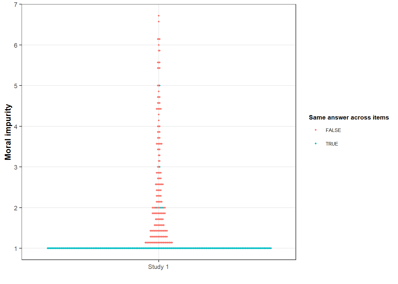
Anomaly 3: bunching on networking intentions
data3a <- data3a %>%
  rowwise() %>%
  mutate(sdNI = sd(c(NI1, NI2, NI3, NI4))) %>%
  as.data.frame()

data3a <- data3a %>% mutate(NIsingleanswer = ifelse(sdNI == 0, T, F))

ggplot(data = data3a, aes(x = conditions, y = NI, col = NIsingleanswer)) +
  geom_beeswarm(size = 1, cex = .30) +
  theme_bw() +
  ggtitle("Study 3A") +
  labs(
    x = "Conditions",
    y = "Networking intentions"
  ) +
  theme(
    plot.title = element_text(hjust = 0.5, size = 12, face = "bold"),
    axis.title.x = element_text(size = 10, face = "bold"), axis.text.x = element_text(size = 8),
    axis.title.y = element_text(size = 10, face = "bold"), axis.text.y = element_text(size = 8),
    legend.title = element_text(size = 8, face = "bold"), legend.text = element_text(size = 6)
  ) +
  scale_y_continuous(breaks = seq(1, 7, 1), minor_breaks = NULL) +
  scale_colour_discrete(name = "Same answer across items")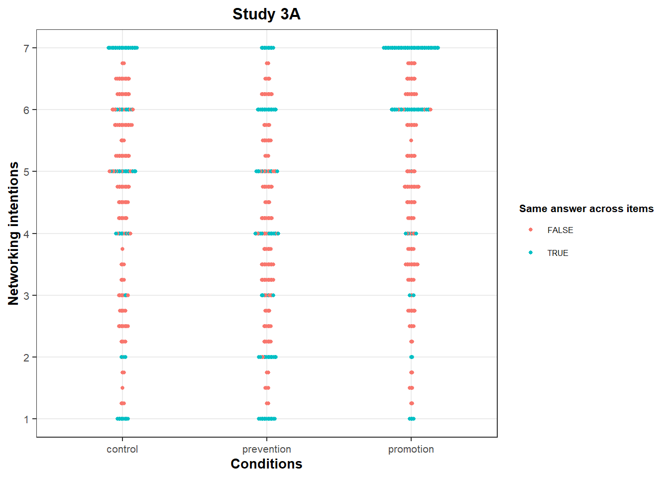
data3b <- data3b %>%
  rowwise() %>%
  mutate(sdNI = sd(c(NI1, NI2, NI3, NI4))) %>%
  as.data.frame()

data3b <- data3b %>% mutate(NIsingleanswer = ifelse(sdNI == 0, T, F))

ggplot(data = data3b, aes(x = conditions, y = NI, col = NIsingleanswer)) +
  geom_beeswarm(size = 1, cex = .30) +
  theme_bw() +
  ggtitle("Study 3B") +
  labs(
    x = "Conditions",
    y = "Networking intentions"
  ) +
  theme(
    plot.title = element_text(hjust = 0.5, size = 12, face = "bold"),
    axis.title.x = element_text(size = 10, face = "bold"), axis.text.x = element_text(size = 8),
    axis.title.y = element_text(size = 10, face = "bold"), axis.text.y = element_text(size = 8),
    legend.title = element_text(size = 8, face = "bold"), legend.text = element_text(size = 6)
  ) +
  scale_y_continuous(breaks = seq(1, 7, 1), minor_breaks = NULL) +
  scale_colour_discrete(name = "Same answer across items")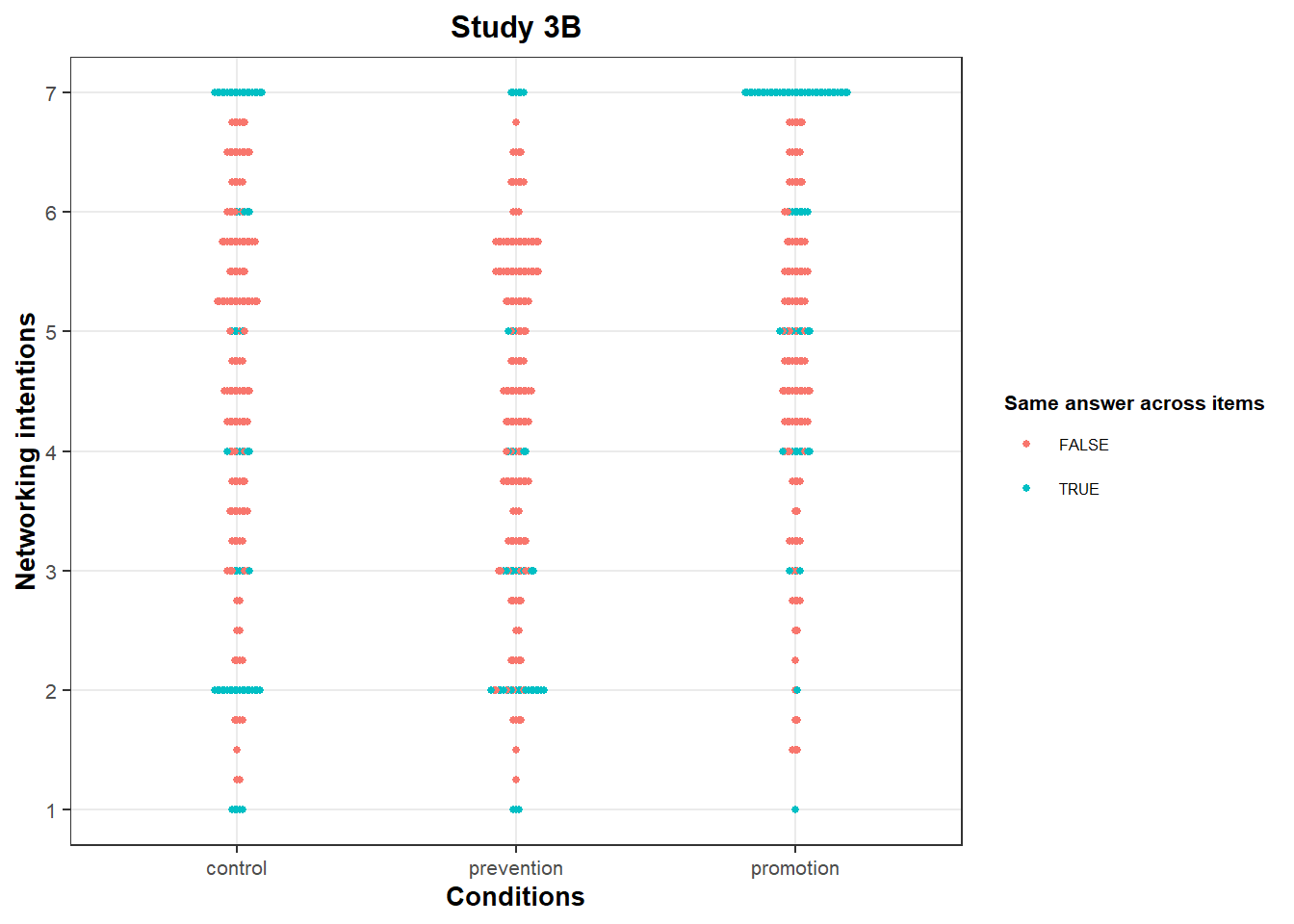
On this scale, the clustering at 7 is compatible with a ceiling effect.
However, we again see bunching at other integer values, albeit less pronounced:
In Study 3A, we see an over-representation of integer values in the “prevention” condition. This is particularly visible on the values “2” and “6”: There are many of them compared to other close values (e.g., 1.75 or 2.25). We also see bunching at “6” in the “promotion” condition, particularly compared to other close values (e.g., 5.75 or 6.25).
In Study 3B, the value “2” is over-represented in the “prevention” and “control” conditions, particularly compared to other close values (e.g., 1.75 or 2.25).
Anomaly 4: bunching on both scales
This “bunching” is unexpected: There is little reason why many participants would converge on the same values. However, it may still reflect a coincidence.
What is even more surprising is that the participants often converge on the same “pairs of values” on the “Moral Impurity” and “Networking Intentions” scales.
Consider Study 3A first:
data3a$NIf <- factor(round(data3a$NI, 2), levels = round(seq(1, 7, 1 / 4), 2))
data3a$MIf <- factor(round(data3a$MI, 2), levels = round(seq(1, 7, 1 / 7), 2))

options(repr.plot.width = 20, repr.plot.height = 10)

freqTable <- ggplot(data3a, aes(MIf, NIf)) +
  geom_bin2d() +
  stat_bin2d(geom = "text", aes(label = ..count..)) +
  scale_fill_gradient(low = "yellow", high = "red", trans = "log", breaks = c(0, 1, 5, 10, 30)) +
  ggtitle("Study 3A") +
  theme(
    plot.title = element_text(hjust = 0.5, size = 14, face = "bold"),
    axis.title.x = element_text(size = 12, face = "bold"),
    axis.title.y = element_text(size = 12, face = "bold"),
    axis.text.x = element_text(size = 5),
    axis.text.y = element_text(size = 7),
    legend.position = "none"
  ) +
  scale_x_discrete(drop = FALSE) +
  scale_y_discrete(drop = FALSE) +
  xlab("Moral Impurity") +
  ylab("Networking Intentions")

integer <- seq(1, 50, by = 7)
for (i in integer) {
  freqTable <- freqTable + geom_vline(xintercept = i + .5, linetype = "dashed", color = "blue") + geom_vline(xintercept = i - .5, linetype = "dashed", color = "blue")
}

integer <- seq(1, 28, by = 4)
for (i in integer) {
  freqTable <- freqTable + geom_hline(yintercept = i + .5, linetype = "dashed", color = "blue") + geom_hline(yintercept = i - .5, linetype = "dashed", color = "blue")
}

freqTable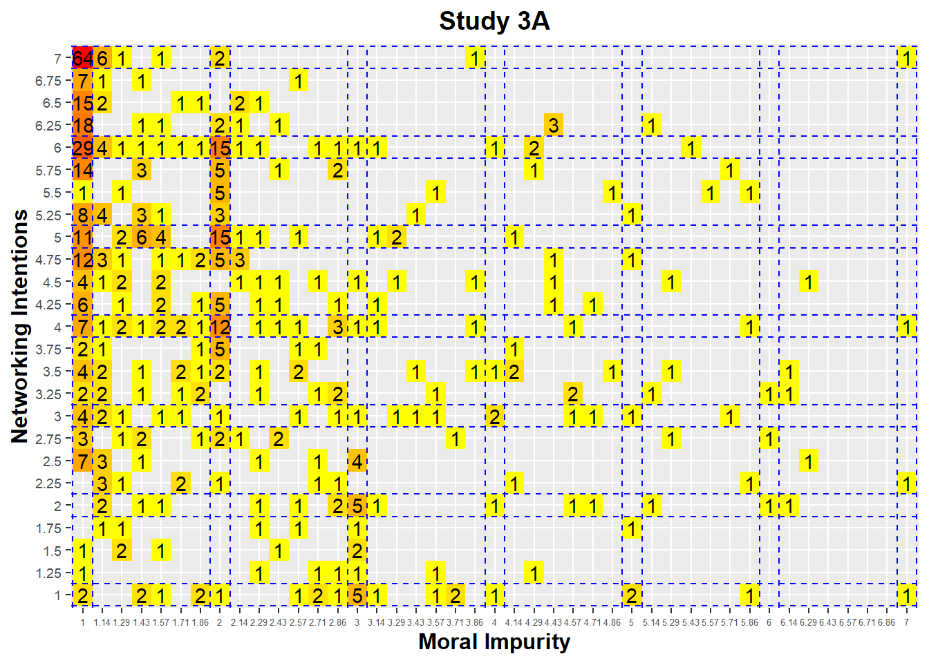
This heatmap presents the number of responses associated with each pair of (Moral Impurity, Networking Intentions) score. For instance, we can see that 64 participants gave a score of “1” on the “Moral Impurity” scale, and a score of “7” on the “Networking Intentions” scale. This is consistent with the ceiling and floor effects observed on those two variables.
However, what is surprising is the large number of respondents (15) who answer (2, 6) on the scales of Moral Impurity and Networking Intentions, while there are fewer responses in the vicinity of this pair. We see the same clustering at (2, 5) and at (2, 4), with again an over-representation of values at these points.
To make sure that it is not again a coincidence, we can inspect the data of Study 3B:
data3b$NIf <- factor(round(data3b$NI, 2), levels = round(seq(1, 7, 1 / 4), 2))
data3b$MIf <- factor(round(data3b$MI, 2), levels = round(seq(1, 7, 1 / 7), 2))

options(repr.plot.width = 20, repr.plot.height = 10)

freqTable <- ggplot(data3b, aes(MIf, NIf)) +
  geom_bin2d() +
  stat_bin2d(geom = "text", aes(label = ..count..)) +
  scale_fill_gradient(low = "yellow", high = "red", trans = "log", breaks = c(0, 1, 5, 10, 30)) +
  ggtitle("Study 3B") +
  theme(
    plot.title = element_text(hjust = 0.5, size = 14, face = "bold"),
    axis.title.x = element_text(size = 12, face = "bold"),
    axis.title.y = element_text(size = 12, face = "bold"),
    axis.text.x = element_text(size = 5),
    axis.text.y = element_text(size = 7),
    legend.position = "none"
  ) +
  scale_x_discrete(drop = FALSE) +
  scale_y_discrete(drop = FALSE) +
  xlab("Moral Impurity") +
  ylab("Networking Intentions")

integer <- seq(1, 50, by = 7)
for (i in integer) {
  freqTable <- freqTable + geom_vline(xintercept = i + .5, linetype = "dashed", color = "blue") + geom_vline(xintercept = i - .5, linetype = "dashed", color = "blue")
}

integer <- seq(1, 28, by = 4)
for (i in integer) {
  freqTable <- freqTable + geom_hline(yintercept = i + .5, linetype = "dashed", color = "blue") + geom_hline(yintercept = i - .5, linetype = "dashed", color = "blue")
}

freqTable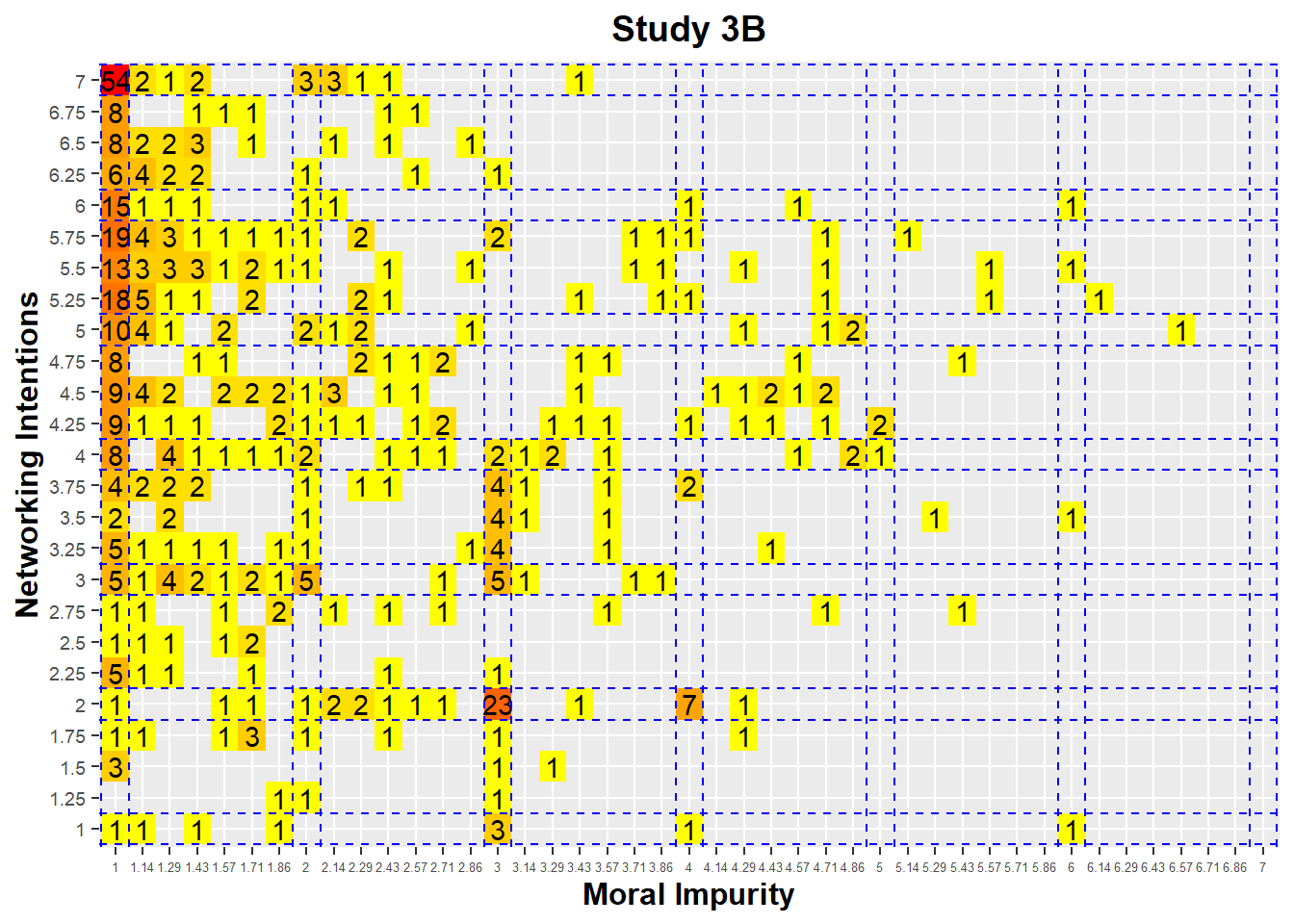
We again see bunching up at (1, 7), with 54 persons choosing this combination of responses in the data. This is again consistent with the ceiling and floor effects observed on these two variables.
In this data, the bunching up is even more dramatic: We see a very large number of respondents (23) who answer (3, 2) on the scales of Moral Impurity and Networking Intentions, while there are very few responses in the vicinity of this pair. We also see bunching at the (4, 2) pair, with 7 responses isolated from others.
Anomaly 5: the mediation pattern is driven by the bunched-up values
The authors hypothesize and find a mediation: A prevention focus is associated with higher levels of moral impurity that are then associated with lower levels of networking intentions. This pattern is found in both studies:
options(repr.plot.width = 6.38, repr.plot.height = 4)

ggplot(data = data3a, aes(x = MI, y = NI)) +
  theme_bw() +
  geom_jitter(size = 1, width = .02, height = .04, alpha = .5, stroke = F) +
  geom_smooth(method = "lm", formula = y ~ x) +
  ggtitle("Study 3A") +
  labs(
    x = "Moral Impurity",
    y = "Netwokring Intentions"
  ) +
  theme(
    plot.title = element_text(hjust = 0.5, size = 14, face = "bold"),
    axis.title.x = element_text(size = 12, face = "bold"),
    axis.title.y = element_text(size = 12, face = "bold"),
    axis.text = element_text(size = 10)
  ) +
  scale_y_continuous(breaks = seq(1, 7, 1), minor_breaks = NULL) +
  scale_x_continuous(breaks = seq(1, 7, 1), minor_breaks = NULL)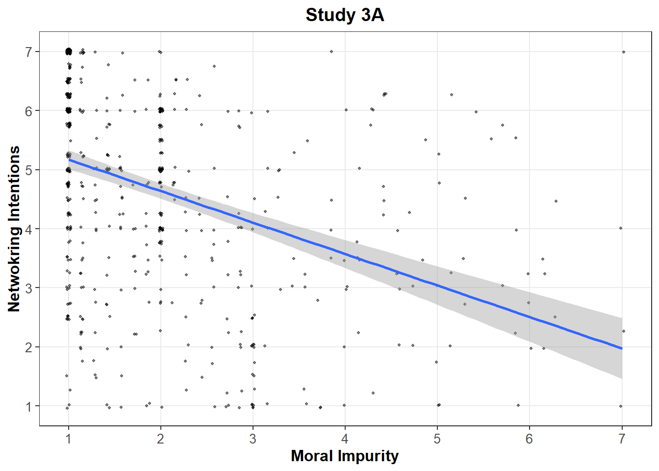
options(repr.plot.width = 6.38, repr.plot.height = 4)

ggplot(data = data3b, aes(x = MI, y = NI)) +
  theme_bw() +
  geom_jitter(size = 1, width = .02, height = .04, alpha = .5, stroke = F) +
  geom_smooth(method = "lm", formula = y ~ x) +
  ggtitle("Study 3B") +
  labs(
    x = "Moral Impurity",
    y = "Netwokring Intentions"
  ) +
  theme(
    plot.title = element_text(hjust = 0.5, size = 14, face = "bold"),
    axis.title.x = element_text(size = 12, face = "bold"),
    axis.title.y = element_text(size = 12, face = "bold"),
    axis.text = element_text(size = 10)
  ) +
  scale_y_continuous(breaks = seq(1, 7, 1), minor_breaks = NULL) +
  scale_x_continuous(breaks = seq(1, 7, 1), minor_breaks = NULL)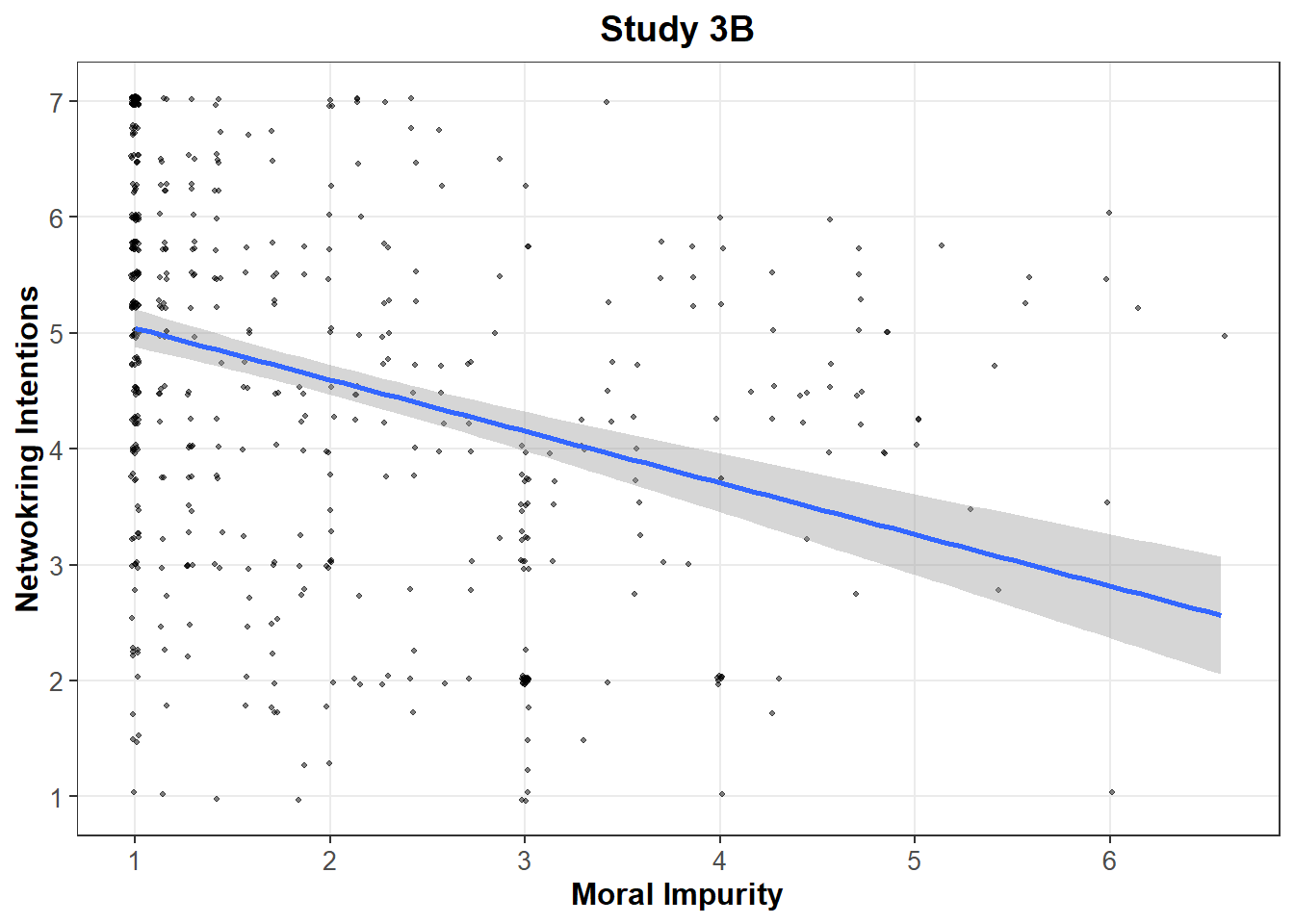
On both panels, it appears that the “bunched-up values” previously documented appear to drive this relationship.
We can bin the Moral Impurity scale in six buckets to confirm this intuition:
x <- data3a$MI
data3a$MIbins <- factor(case_when(
  x == 1 ~ "MI = 1",
  x < 2 ~ "1 < MI < 2",
  x == 2 ~ "MI = 2",
  x < 3 ~ "2 < MI < 3",
  x == 3 ~ "MI = 3",
  x > 3 ~ "MI > 3"
), levels = c("MI = 1", "1 < MI < 2", "MI = 2", "2 < MI < 3", "MI = 3", "MI > 3"))

meanCI <- data3a %>%
  group_by(MIbins) %>%
  summarise(
    n = n(),
    mean = mean(NI),
    sd = sd(NI)
  ) %>%
  mutate(se = sd / sqrt(n)) %>%
  mutate(ci = se * qt((1 - 0.05) / 2 + .5, n - 1))

ggplot(meanCI, aes(x = MIbins, y = mean)) +
  geom_errorbar(aes(ymin = mean - ci, ymax = mean + ci), width = .1) +
  geom_point(size = 2) +
  ggtitle("Study 3A") +
  theme_bw() +
  xlab("Moral Impurity (binned)") +
  ylab("Networking intentions") +
  theme(
    plot.title = element_text(hjust = 0.5, size = 12, face = "bold"),
    axis.title.x = element_text(size = 10, face = "bold"), axis.text.x = element_text(size = 8),
    axis.title.y = element_text(size = 10, face = "bold"), axis.text.y = element_text(size = 8)
  ) +
  scale_y_continuous(minor_breaks = NULL)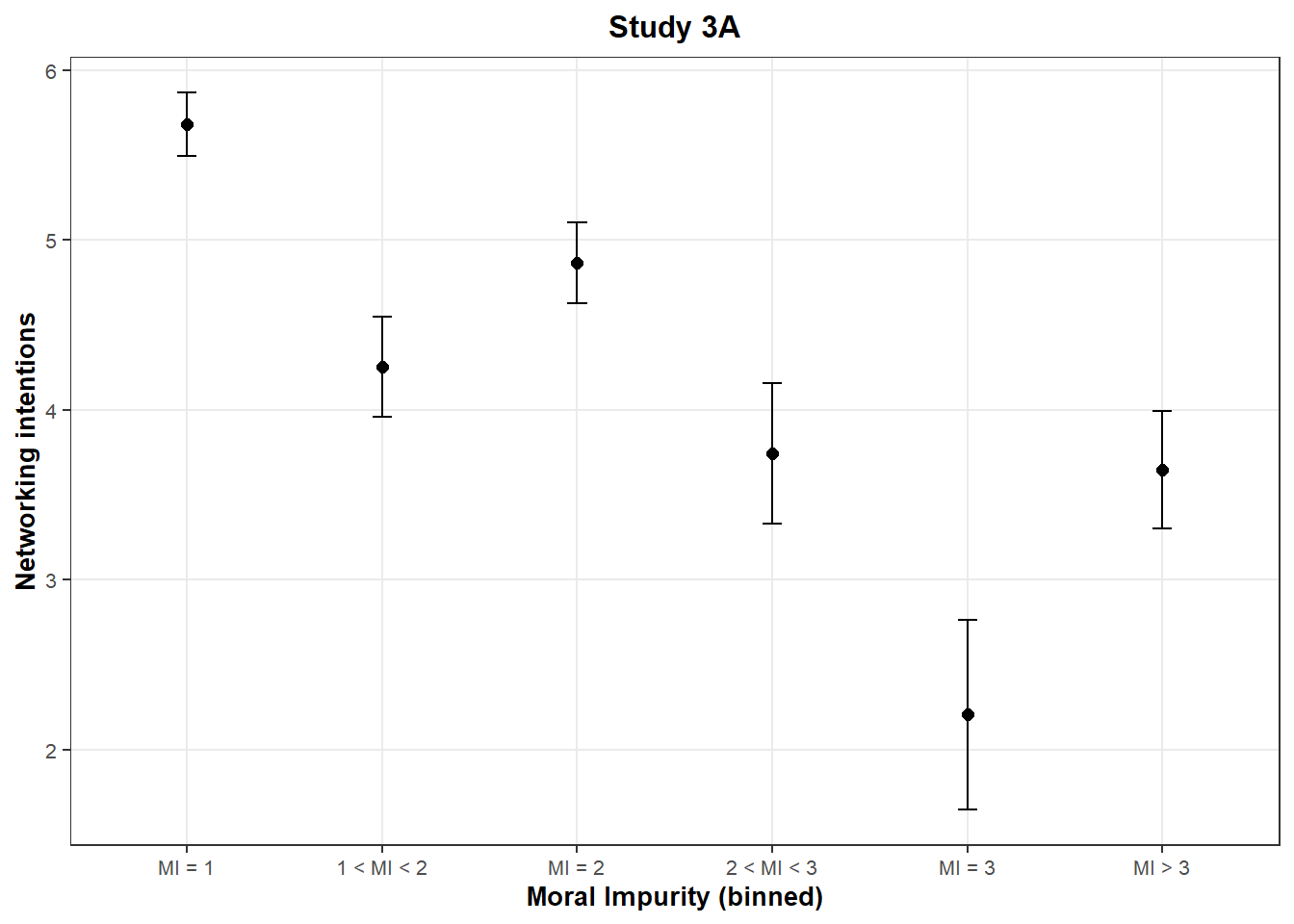
x <- data3b$MI
data3b$MIbins <- factor(case_when(
  x == 1 ~ "MI = 1",
  x < 2 ~ "1 < MI < 2",
  x == 2 ~ "MI = 2",
  x < 3 ~ "2 < MI < 3",
  x == 3 ~ "MI = 3",
  x > 3 ~ "MI > 3"
), levels = c("MI = 1", "1 < MI < 2", "MI = 2", "2 < MI < 3", "MI = 3", "MI > 3"))

meanCI <- data3b %>%
  group_by(MIbins) %>%
  summarise(
    n = n(),
    mean = mean(NI),
    sd = sd(NI)
  ) %>%
  mutate(se = sd / sqrt(n)) %>%
  mutate(ci = se * qt((1 - 0.05) / 2 + .5, n - 1))

ggplot(meanCI, aes(x = MIbins, y = mean)) +
  geom_errorbar(aes(ymin = mean - ci, ymax = mean + ci), width = .1) +
  geom_point(size = 2) +
  ggtitle("Study 3B") +
  theme_bw() +
  xlab("Moral Impurity (binned)") +
  ylab("Networking intentions") +
  theme(
    plot.title = element_text(hjust = 0.5, size = 12, face = "bold"),
    axis.title.x = element_text(size = 10, face = "bold"), axis.text.x = element_text(size = 8),
    axis.title.y = element_text(size = 10, face = "bold"), axis.text.y = element_text(size = 8)
  ) +
  scale_y_continuous(minor_breaks = NULL)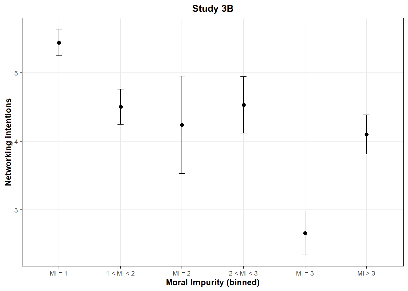
These graphs reveal a surprising pattern: The networking intentions of participants who answered exactly “3” on the scale of moral impurity are much lower than the networking intentions of other participants, even when compared to participants who have higher levels of moral impurity (x > 3). This runs counter the authors’ hypothesis, and is observed in both studies.
Another way to look at this pattern is to notice that the integer values are driving the entirety of the association between Moral Impurity and Networking Intentions.
When we consider instead the non-integer values, we see a much weaker, non-significant or barely significant, association between the two variables:
data3a$intMI <- data3a$MI %% 1 == 0

options(repr.plot.width = 7, repr.plot.height = 4)

ggplot(data = data3a, aes(x = MI, y = NI, col = intMI)) +
  theme_bw() +
  geom_jitter(size = 1, width = .02, height = .04, alpha = .5, stroke = F) +
  geom_smooth(method = "lm", formula = y ~ x) +
  ggtitle("Study 3A") +
  labs(
    x = "Moral Impurity",
    y = "Netwokring Intentions"
  ) +
  theme(
    plot.title = element_text(hjust = 0.5, size = 12, face = "bold"),
    axis.title.x = element_text(size = 10, face = "bold"),
    axis.title.y = element_text(size = 10, face = "bold"),
    axis.text = element_text(size = 10),
    legend.title = element_text(size = 8, face = "bold"), legend.text = element_text(size = 6)
  ) +
  scale_y_continuous(breaks = seq(1, 7, 1), minor_breaks = NULL) +
  scale_x_continuous(breaks = seq(1, 7, 1), minor_breaks = NULL) +
  scale_colour_discrete(name = "Moral impurity is int.")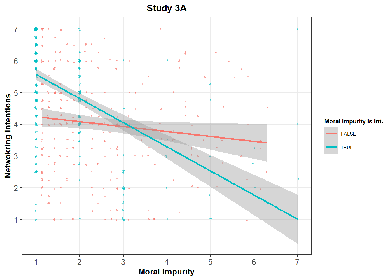
Regression table:
model <- lm(NI ~ MI * intMI, data = data3a)
model <- broom::tidy(model) %>%
  mutate(coeff = c("Intercept", "Moral Impurity (Non-Int)", "Is Integer?", "Moral Impurity x Integer")) %>%
  select(coeff, estimate, p.value)

model <- model %>% mutate_at(2, round, 2)
model <- as.data.frame(model)
colnames(model) <- c("Coefficient", "Estimate", "p.value")

model
## Coefficient Estimate p.value
## 1 Intercept 4.40 3.364294e-78
## 2 Moral Impurity (Non-Int) -0.16 2.775910e-02
## 3 Is Integer? 1.94 2.517436e-14
## 4 Moral Impurity x Integer -0.61 6.868950e-09data3b$intMI <- data3b$MI %% 1 == 0
options(repr.plot.width = 7, repr.plot.height = 4)
ggplot(data = data3b, aes(x = MI, y = NI, col = intMI)) +
theme_bw() +
geom_jitter(size = 1, width = .02, height = .04, alpha = .5, stroke = F) +
geom_smooth(method = "lm", formula = y ~ x) +
ggtitle("Study 3B") +
labs(
x = "Moral Impurity",
y = "Netwokring Intentions"
) +
theme(
plot.title = element_text(hjust = 0.5, size = 12, face = "bold"),
axis.title.x = element_text(size = 10, face = "bold"),
axis.title.y = element_text(size = 10, face = "bold"),
axis.text = element_text(size = 10),
legend.title = element_text(size = 8, face = "bold"), legend.text = element_text(size = 6)
) +
scale_y_continuous(breaks = seq(1, 7, 1), minor_breaks = NULL) +
scale_x_continuous(breaks = seq(1, 7, 1), minor_breaks = NULL) +
scale_colour_discrete(name = "Moral impurity is int.")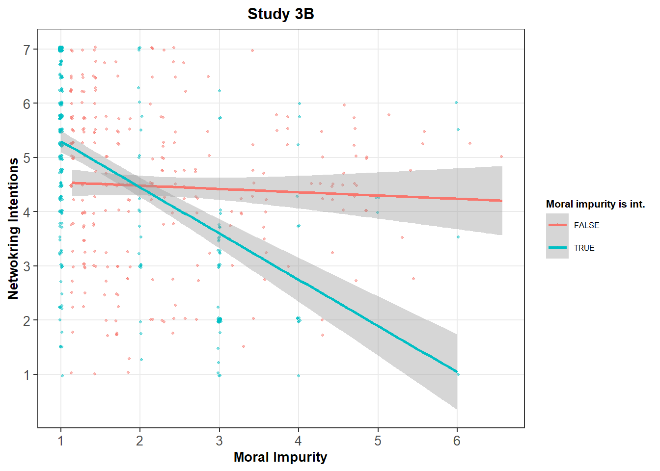
Regression table:
model <- lm(NI ~ MI * intMI, data = data3b)
model <- broom::tidy(model) %>%
  mutate(coeff = c("Intercept", "Moral Impurity (Non-Int)", "Is Integer?", "Moral Impurity x Integer")) %>%
  select(coeff, estimate, p.value)

model %>% mutate_at(2, round, 2)
## # A tibble: 4 × 3
## coeff estimate p.value
## <chr> <dbl> <dbl>
## 1 Intercept 4.61 3.15e-85
## 2 Moral Impurity (Non-Int) -0.06 4.21e- 1
## 3 Is Integer? 1.55 1.04e- 9
## 4 Moral Impurity x Integer -0.79 7.77e-13model <- as.data.frame(model)
colnames(model) <- c("Coefficient", "Estimate", "p.value")
model## Coefficient Estimate p.value
## 1 Intercept 4.60582170 3.151740e-85
## 2 Moral Impurity (Non-Int) -0.06068862 4.208058e-01
## 3 Is Integer? 1.54880845 1.037728e-09
## 4 Moral Impurity x Integer -0.79133863 7.765745e-13The interaction term is significant (p < .001) in both studies, suggesting that the behavior of participants who answer integer values is significantly different from the behavior of other participants.
Anomaly 6: sentiment analysis
As previously mentioned, in study 3A, we observed many “all 1s” responses on the “Moral Impurity” scale in all conditions, but the “Prevention” condition. In fact, in this condition, we observed many “all 2s” and “all 3s” responses.
A potential explanation might be that the “all 1s” responses in the “Prevention” condition have been altered in “all 2s” or “all 3s” responses to fit the hypothesis of the authors.
To check whether these “all 2s”, “all 3s” responses might in fact be “all 1s”, we can use the text participants wrote about networking. Indeed, in study 3A, participants were asked to read a story describing someone networking, to put themselves in the shoes of this person, and to reflect on networking by writing a few words about it.
The idea is that the text participants wrote should reflect how positive or negative they felt about the networking event they described. If they feel positive about networking, the valence of their text should be positive, and their level of moral impurity should be low. On the contrary, if they feel negative about networking, the valence of their text should be negative, and their level of moral impurity should be high.
To capture the valence of participants’ text, we can run a sentiment analysis using the VADER package in R. VADER will give us a score between +1 (most positive) and -1 (most negative) capturing the attitude, sentiments, emotions and evaluation of the writer about networking.
We should therefore see that the higher the Vader score (i.e., more positive sentiment), the lower the moral impurity, and vice versa (the lower the Vader score, the more negative the sentiment, the higher the moral impurity).
However, our prediction is that participants who responded “all 2s” or “all 3s” (which, again, we suspect were originally “1s” in the data) in the “Prevention” condition will have a high Vader score (i.e., be associated with a text that has positive sentiments).
# Modify unreadable characters
data3a$words2_cond[26] = gsub("it\x82\xc4\xf4s", "it's", data3a$words2_cond[26])
data3a$words2_cond[242] = gsub("didn\x82\xc4\xf4t", "didn't", data3a$words2_cond[242])

# Compute the Vader score
data3a$vader_score <- vader_df(data3a$words2_cond)

# Compute the standard deviation of each response to the Moral Impurity scale
data3a$MIsd <- apply(data3a[,7:13], 1, sd)

# Identify which responses might have been tampered (when the mean response is 2 or 3, the standard deviation of this mean is 0, and the condition is "prevention").
data3a <- data3a %>% mutate(tampered = ifelse((MIsd==0) & (MI==2 | MI==3) & (conditions=='prevention'), 1, 0))

# Compute the average Vader score of these tampered responses
subdata <- data3a %>% filter(data3a$tampered== 1)
sample <- as.data.frame(table(subdata$MI))
a <- sample[1, 2]
b <- sample[2 ,2]
means <- subdata %>%
  group_by(MI) %>%
  dplyr::summarize(VaderScore = round(mean(vader_score$compound), 2))
means <- means %>% mutate(n=c(a, b))
means$MI <- as.character(means$MI)

# Compute the average Vader score of the non-tampered response for different average value of Moral Impurity
subdata <- data3a %>% filter(data3a$tampered == 0)

## For MI = 1
bean1 <- subdata %>% filter(subdata$MI == 1)
c <- nrow(bean1)
meanb1 <- bean1 %>%
  group_by(MI) %>%
  dplyr::summarize(VaderScore = round(mean(vader_score$compound), 2))
meanb1 <- meanb1 %>% mutate(n=c)
meanb1$MI <- as.character(meanb1$MI)

## For MI = ]1; 2[
bean2 <- subdata %>% filter(subdata$MI > 1 & subdata$MI < 2)
d <- nrow(bean2)
meanb2 <- bean2 %>%
  dplyr::summarize(VaderScore = round(mean(vader_score$compound),2))
meanb2 <- meanb2 %>% mutate(n=d)
meanb2 <- meanb2 %>% mutate(MI = "]1; 2[", .before=VaderScore)

## For MI = [2; 3[
bean3 <- subdata %>% filter(subdata$MI >= 2 & subdata$MI < 3)
e <- nrow(bean3)
meanb3 <- bean3 %>%
  dplyr::summarize(VaderScore = round(mean(vader_score$compound), 2))
meanb3 <- meanb3 %>% mutate(n=e)
meanb3 <- meanb3 %>% mutate(MI = "[2; 3[", .before=VaderScore)

## For MI >= 3
bean4 <- subdata %>% filter(subdata$MI >= 3)
f <- nrow(bean4)
meanb4 <- bean4 %>%
  dplyr::summarize(VaderScore = round(mean(vader_score$compound), 2))
meanb4 <- meanb4 %>% mutate(n=f)
meanb4 <- meanb4 %>% mutate(MI = ">= 3", .before=VaderScore)

# Outcome
final <- bind_rows(meanb1, meanb2, means[1,], meanb3, means[2,], meanb4) %>% mutate(Tampered = c(0, 0, 1, 0, 1, 0), MI=factor(MI, levels=c('1', "]1; 2[", "2", "[2; 3[", "3", ">= 3")))

final <- as.data.frame(final)
colnames(final) <- c("Moral impurity", "Vader score", "n", "Tampered data")
final
## Moral impurity Vader score n Tampered data
## 1 1 0.48 222 0
## 2 ]1; 2[ 0.33 122 0
## 3 2 0.53 61 1
## 4 [2; 3[ 0.07 84 0
## 5 3 0.62 18 1
## 6 >= 3 -0.01 92 0data3a$sa <- factor(case_when(
(data3a$MI == 1 & data3a$tampered == 0) ~ "1",
(data3a$MI > 1 & data3a$MI < 2 & data3a$tampered == 0) ~ "]1; 2[",
(data3a$MI == 2 & data3a$tampered == 1) ~ "2",
(data3a$MI >= 2 & data3a$MI < 3 & data3a$tampered == 0) ~ "[2; 3[",
(data3a$MI == 3 & data3a$tampered == 1) ~ "3",
(data3a$MI >= 3 & data3a$tampered == 0) ~ ">= 3"
), levels=c("1", "]1; 2[", "2", "[2; 3[", "3", ">= 3"))
meanCI <- data3a %>%
group_by(sa) %>%
summarise(
n = n(),
mean = mean(vader_score$compound),
sd = sd(vader_score$compound)
) %>%
mutate(se = sd / sqrt(n)) %>%
mutate(ci = se * qt((1 - 0.05) / 2 + .5, n - 1)) %>%
mutate(Tampered = c(0, 0, 1, 0, 1, 0))
meanCI$Tampered <- factor(meanCI$Tampered, levels=c("0", "1"))
ggplot(meanCI, aes(x = sa, y = mean)) +
geom_errorbar(aes(ymin = mean - ci, ymax = mean + ci), width = .1) +
geom_point(aes(color=Tampered), size = 2.5) +
scale_colour_manual(name = "Tampered Data", values = c("blue", "red")) +
ggtitle("Study 3A") +
theme_bw() +
xlab("Moral Impurity (binned)") +
ylab("Vader Score") +
theme(
plot.title = element_text(hjust = 0.5, size = 12, face = "bold"),
axis.title.x = element_text(size = 10, face = "bold"),
axis.text.x = element_text(size = 8),
axis.title.y = element_text(size = 10, face = "bold"),
axis.text.y = element_text(size = 8)
) +
scale_y_continuous(minor_breaks = NULL)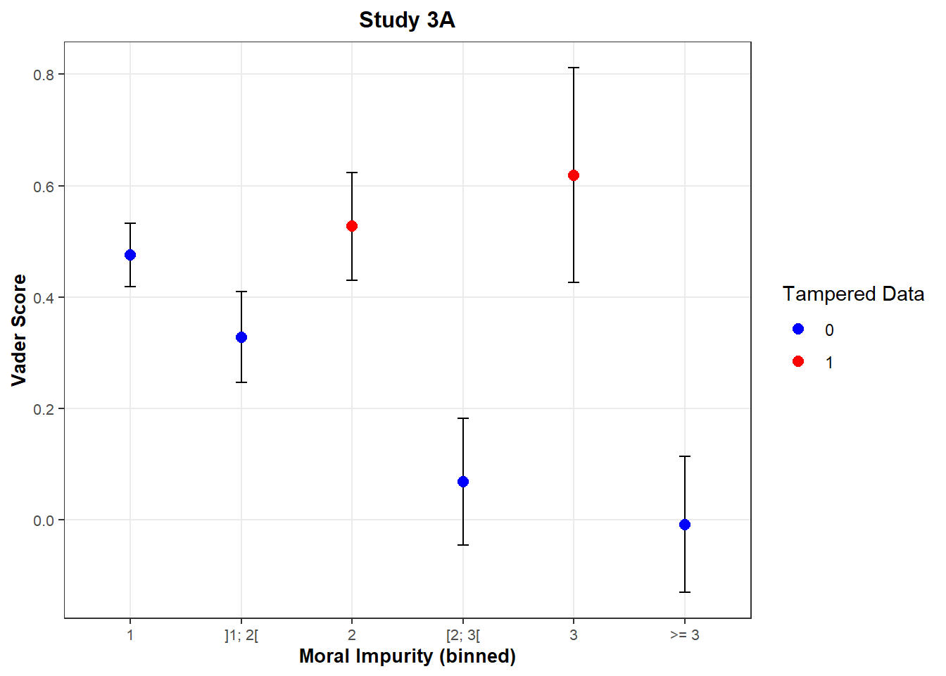
The presumably tampered responses have the highest Vader score on average (more positive sentiments towards networking). In particular, while for non-tampered responses, a level of moral impurity around 2, 3 is associated with a Vader score between -0.01 and 0.33, for the tampered responses, a level of moral impurity of 2, 3 is associated with an average weighted Vader score of 0.55.
For the rest of responses, the Vader score behaves as expected: It decreases as the level of Moral Impurity increases.
Zoé Ziani
PhD in Organizational Behavior