In Figures
The author has an impressive academic vita: 19 pages, an H-index of 87, roughly 33 000 citations…
To understand the scope of the issue, I built a dataset (from her website) of her papers including:
Year of publication
Co-authors and their affiliation
Journals
Here is what I learnt from it.
#libraries
library(dplyr)
library(stringr)
library(tidyr)
library(tidyverse)
library(ggplot2)
library(lubridate)
# DATASET
## Dataset built from her website
data <- read.csv("GinoNetwork_myversion_cleaned.csv")
## Separation of authors on each paper
cdata <- data %>% mutate(Coauthors=str_split(Authors, fixed("., "))) %>% unnest(Coauthors)
cdata$Coauthors <- gsub('& ','',cdata$Coauthors)
cdata$Coauthors[-length(cdata$Coauthors)] <- paste0(cdata$Coauthors[-length(cdata$Coauthors)], '.')
cdata$Coauthors <- gsub('..','.',cdata$Coauthors, fixed = TRUE)
# AUTORSHIP
## Position of authorship on each paper
Gorder_data <- cdata %>% group_by(Title) %>% mutate(Position=row_number()) %>% filter(Coauthors == 'Gino, F.')
Gorder_data <- Gorder_data[,c("Title","Position")]
## Merge the position dataframe with the whole dataframe
cdata <- merge(cdata, Gorder_data, by="Title")
cdata <- cdata %>% filter(Coauthors != "Gino, F.")
cdata <- cdata[, c(2, 1, 4, 3, 5, 6)]
cdata <- cdata %>% arrange(desc(Year), Title)
# AFFILIATION
## Affiliation of coauthors
schools <- read.csv('Schools.csv')
schools[c('Schools', 'Subschools')] <- str_split_fixed(schools$Schools, ', ', 2)
dataplus <- merge(cdata, schools, by="Coauthors")
dataplus <- dataplus[,-7]
dataplus <- dataplus[, c(2, 3, 4, 5, 1, 7, 8, 6)]
dataplus <- dataplus %>% arrange(desc(Year), Title)Productivity
# PRODUCTIVITY

## Stats on Gino's productivity
stats_year <- dataplus %>% group_by(Year, Title) %>% count()
stats_year <- stats_year %>% group_by(Year) %>% count()
stats_year$Year <- as.character(stats_year$Year)

summary(stats_year$n)
## Min. 1st Qu. Median Mean 3rd Qu. Max.
## 1.000 7.000 8.000 8.294 11.000 15.000## Histogram on Gino's productivity
histo <- ggplot(stats_year, aes(x = n, y = Year)) +
geom_bar(stat = "identity", fill = "chartreuse1") +
theme_bw() +
labs(title = "Productivity per Year", x = "Nber of papers", y = "Year",
caption = "Note. 2010 is the year G got into HBS and got tenured.") +
theme(plot.caption = element_text(hjust = 0)) +
geom_hline(yintercept="2010", linetype="dashed",
color = "red", size=0.5) +
theme(text=element_text(size=15))
histo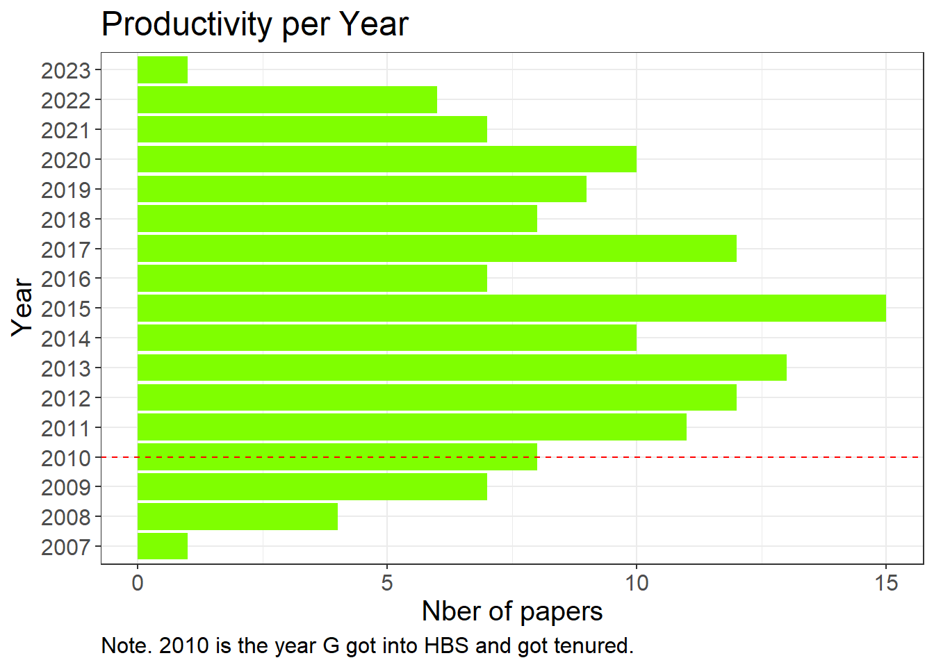
Journals
# FIELDS

## Stats on journals
stats_publi <- data %>% group_by(Source) %>% count()
stats_publi <- stats_publi[order(stats_publi$n),]

filtered_stats_publi <- stats_publi %>% filter(n > 1)

## Histogram on journals
histo <- ggplot(filtered_stats_publi, aes(x = n, y = reorder(Source, n))) +
  geom_bar(stat = "identity", fill = "pink") +
  theme_bw() +
  labs(title = "Papers per Journal", x = "Nber of papers", y = "Journal") +
  theme(text=element_text(size=15))
histo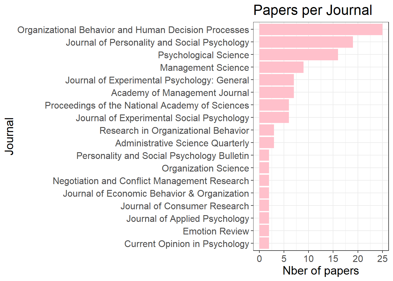
Coauthors
# COAUTHORS

## Stats on Gino's coauthors
stats_coauthors <- dataplus %>% group_by(Coauthors) %>% count()
stats_coauthors <- stats_coauthors[order(stats_coauthors$n),]
filtered_stats_coauthors <- stats_coauthors %>% filter(n > 3)

## Histogram of Gino's coauthors
histo <- ggplot(filtered_stats_coauthors, aes(x = n, y = reorder(Coauthors, n))) +
  geom_bar(stat = "identity", fill = "cadetblue1") +
  theme_bw() +
  labs(title = "Biggest contributors", x = "Nber of papers", y = "Gino's co-authors") +
  theme(text=element_text(size=15))
histo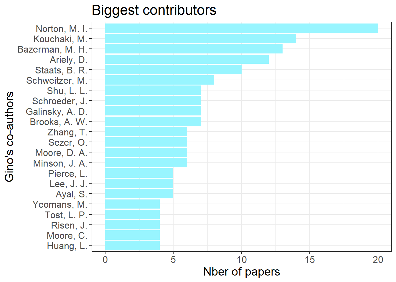
Affiliation
# Stats on Gino's coauthors' affiliation

## Affiliation of her coauthors

stats_schools <- schools %>% group_by(Schools) %>% count()
stats_schools <- stats_schools[order(stats_schools$n),]
filtered_stats_schools <- stats_schools %>% filter(n > 2)

histo1 <- ggplot(filtered_stats_schools, aes(x = n, y = reorder(Schools, n))) +
  geom_bar(stat = "identity", fill = "steelblue1") +
  theme_bw() +
  labs(title = "Affilitation of Gino's Coauthors", x = "Nber of coauthors", y = "Schools")
histo1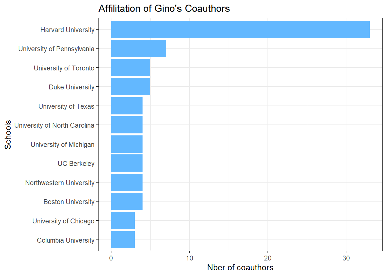
## Affiliation weighted by the nber of papers

w_stats_schools <- dataplus %>% group_by(Schools) %>% count()
w_stats_schools <- w_stats_schools[order(w_stats_schools$n),]
filtered_w_stats_schools <- w_stats_schools %>% filter(n > 5)

histo2 <- ggplot(filtered_w_stats_schools, aes(x = n, y = reorder(Schools, n))) +
  geom_bar(stat = "identity", fill = "steelblue3") +
  theme_bw() +
  labs(title = "Affiliation Weighted by Nber of Papers", x = "Nber of papers", y = "")
histo2
Authorship
# Stats on her position in authorship

# Total
stats_pos_total <- Gorder_data %>% group_by(Position) %>% count()
stats_pos_total$Position <- as.character(stats_pos_total$Position)

# Per year
stats_position <- cdata %>% group_by(Year, Position) %>% count()
stats_position$Position <- as.numeric(stats_position$Position)

pos_per_year <- stats_position %>% group_by(Year) %>% mutate(total=sum(n)) %>% unnest()

pos_per_year <- pos_per_year %>% mutate(pr = n/total)
pos_per_year <- pos_per_year %>% group_by(Year) %>%
  mutate(mean_pos = weighted.mean(Position, pr))

ggplot(pos_per_year, aes(x=Year, y=mean_pos)) + geom_point() +
    scale_x_continuous(breaks = seq(2007, 2023, by = 1), minor_breaks =
                         NULL) +
  scale_y_continuous(breaks = seq(0, 10, by = 1), minor_breaks = NULL) +
  geom_vline(xintercept=2010, linetype="dashed", color = "red", size=0.5) +
  theme_bw() +
  labs(title = "Authorship Over Time", x = "Year", y = "Weighted Average Position in Authorship", caption = "Note. 2010 is the year G got into HBS and got tenured.") +
  theme(plot.caption = element_text(hjust = 0))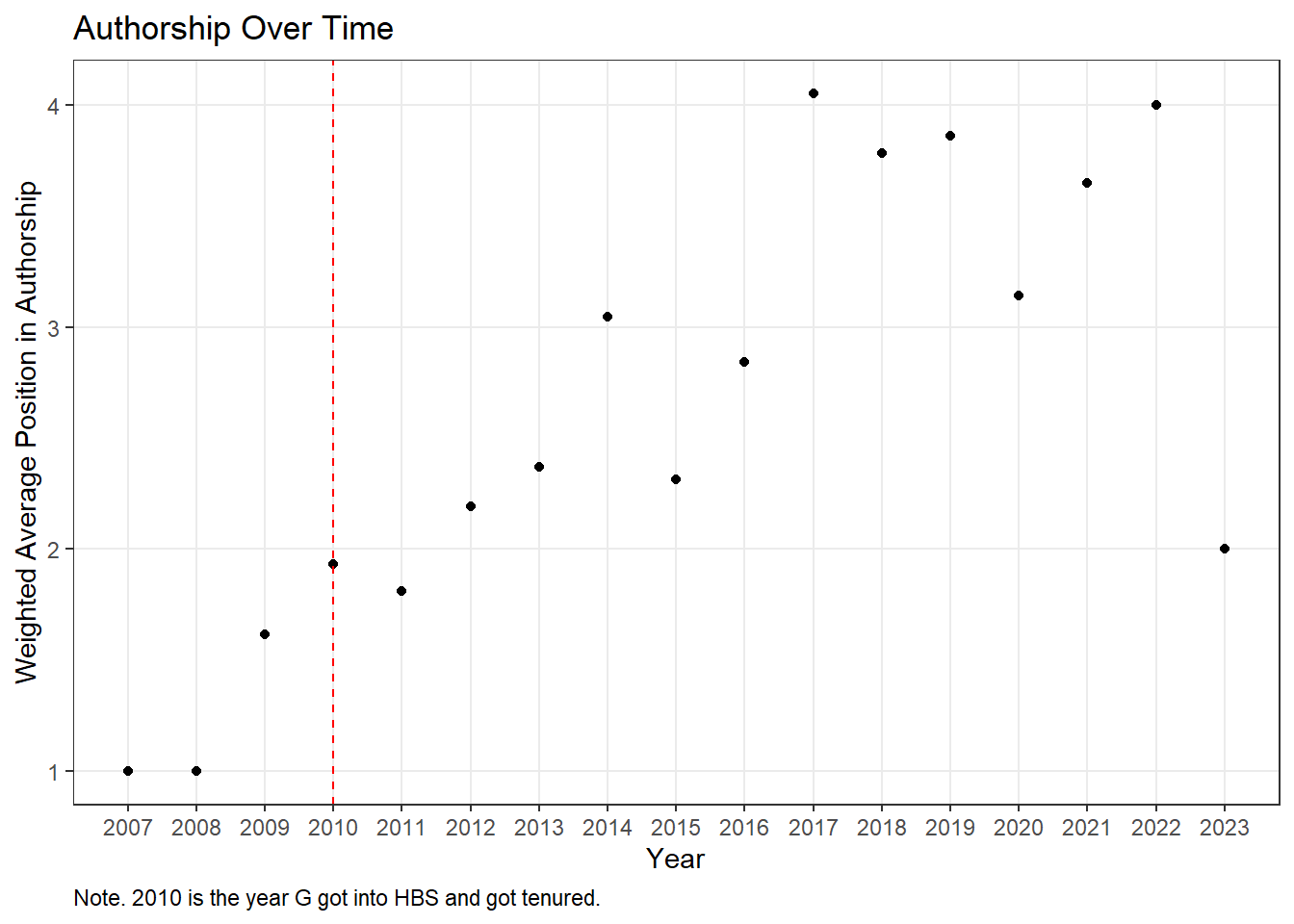
Zoé Ziani
PhD in Organizational Behavior